1.4 The donut shop example
Let’s consider in more details the donut shop example and let’s construct and implement our first simulation model. At this stage, you should not worry about the implementation details. These will be formalized in more details in later chapters.
Let’s make some assumptions:
the queue in the shop is possibly infinite: whenever a customer arrives she will stay in the queue independent of how many customers are already queuing and she will wait until she is served.
customers are served on a first-come, first-served basis.
there are two employees. On average they take the same time to serve a customer. Whenever an employee is free, a customer is allocated to that employee. If both employees are free, either of the two starts serving a customer.
The components of the simulation model are the following:
System state: \(N_C(t)\) number of customers waiting to be served at time \(t\); \(N_E(t)\) number of employees busy at time \(t\).
Resources: customers and employees;
Events: arrival of a customer; service completion by an employee.
Activities: time between a customer arrival and the next; service time by an employee.
Delay: customers’ waiting time in the queue until an employee is available.
From an abstract point of view we have now defined all components of our simulation model. Before implementing, we need to choose the length of the activities. This is usually done using common sense, intuition or historical data. Suppose for instance that the time between the arrival of customers is modeled as an Exponential distribution with parameter 1/3 (that is on average a customer arrives every three minutes) and the service time is modeled as a continuous Uniform distribution between 1 and 5 (on average a service takes three minutes).
With this information we can now implement the workings of our donut shop. It does not matter the specific code itself, we will learn about it in later chapters. At this stage it is only important to notice that we use the simmer package together with the functionalities of magrittr. We simulate our donut shop for two hours.
library(simmer)
library(magrittr)
set.seed(2021)

env <-  simmer("donut shop")

customer <- trajectory("customer") %>% seize("employee", 1) %>%
  timeout(function() runif(1,1,5)) %>% release("employee", 1)

env %>%
  add_resource("employee", 2) %>%
  add_generator("customer", customer, function() rexp(1,1/3))

env %>%
  run(until=120)
The above code creates a simulation of the donut shop for two hours. Next we report some graphical summaries that describe how the system worked.
library(simmer.plot)
library(gridExtra)
p1 <- plot(get_mon_resources(env), metric = "usage", items = "server",step = T)
p2 <- plot(get_mon_arrivals(env), metric = "waiting_time")

grid.arrange(p1,p2,ncol=2)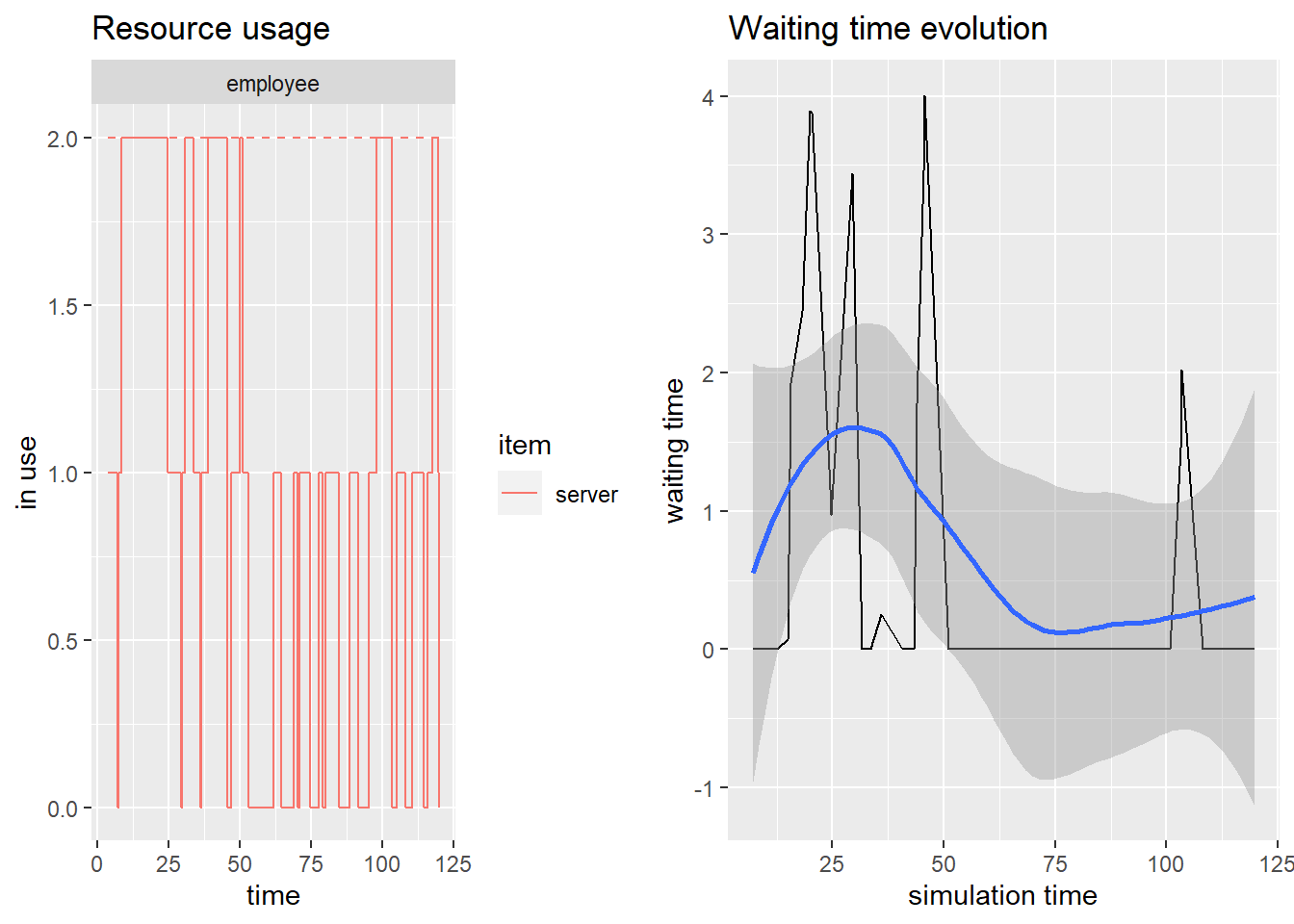
Figure 1.3: Graphical summaries from the simulation of the donut shop
The left plot in Figure 1.3 reports the number of busy employees busy throughout the simulation. We can observe that often no employees were busy, but sometimes both of them are busy. The right plot in Figure 1.3 reports the waiting time of customers throughout the simulation. Most often customers do not wait in our shop and the largest waiting time is of about four minutes.
Some observations:
this is the result of a single simulation where inputs are random and described by a random variable (for instance, Poisson and Uniform). If we were to run the simulation again we would observe different results.
given that we have built the simulation model, it is straightforward to change some of the inputs and observe the results under different conditions. For instance, we could investigate what would happen if we had only one employee. We could also investigate the use of different input parameters for the customer arrival times and the service times.