6.2 Replication

For all previous examples, we ran a unique simulation and observed the results. As we have already learned, these results are affected by randomness and different runs will show different results.

Consider the last simulation we implemented where customers arrive at the shop where we have two counters. We can simulate the system 1000 times using the following code. We will not include log since otherwise the output will become cluttered.

customer <-
  trajectory("Customer's path") %>%
  seize("counter") %>%
  timeout(function() rnorm(1,10,2)) %>%
  release("counter") 


envs <- lapply(1:100, function(i) {
    simmer("shop") %>% 
    add_resource("counter",2) %>%
    add_generator("Customer", customer, function() rexp(1, 1/5)) %>%
    run(until=240)
}
)

Now envs stores the output of simulating the behavior of the shop for 4 hours 100 times.

We can summarize the results of these simulations using the simmer.plot package.

plot(get_mon_resources(envs), metric = "utilization")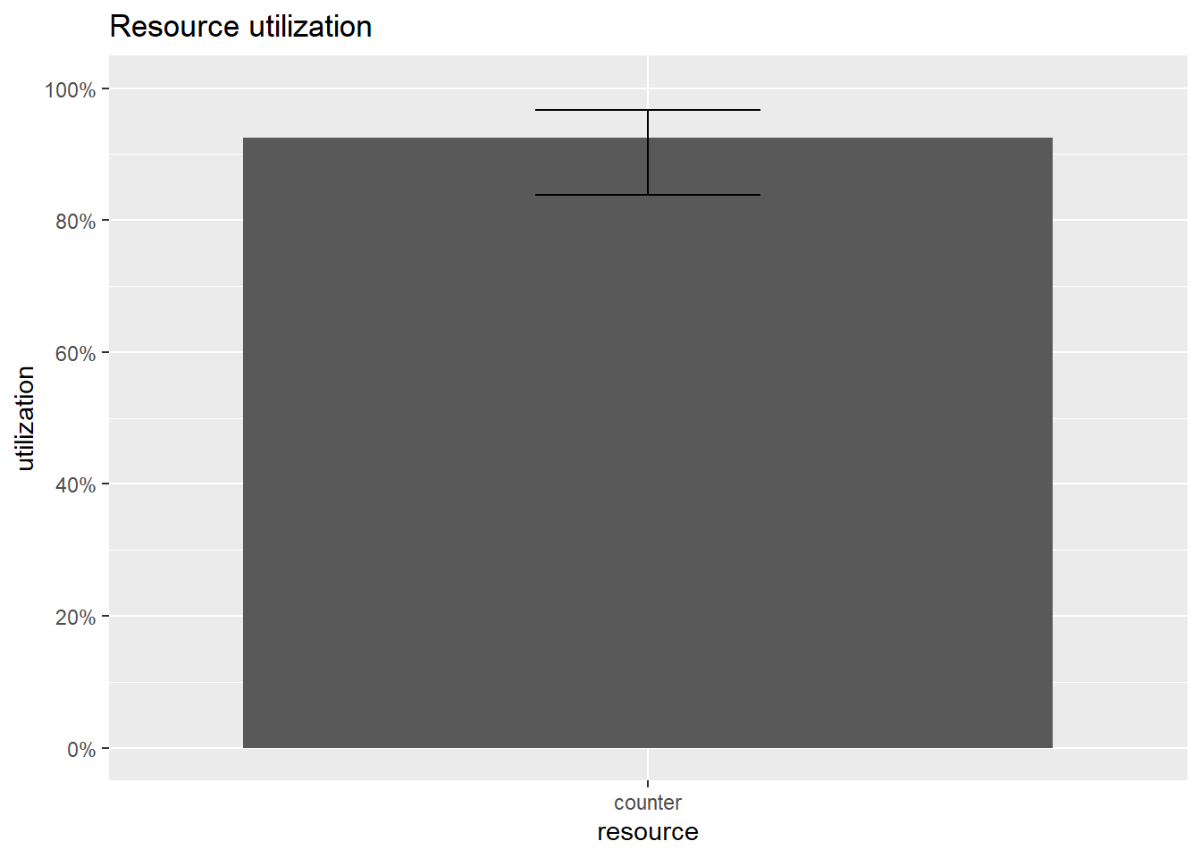

Compared to previous plots we now notice that the output also has something that resembles a boxplot which tells us what was the utilization of the resource in different simulation runs.

We can also assess how busy were the employees in different simulations. As the shop opens the two employees become more and more busy and at the end of the four hours they are busy almost all the time.

plot(get_mon_resources(envs), metric = "usage", items = "server")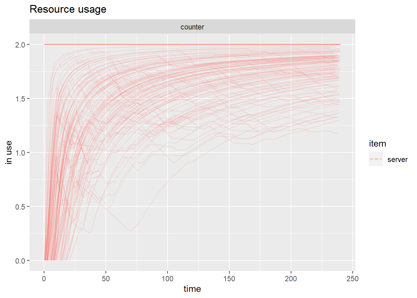

Similarly, we can look at how long do customers queue in our shop.

plot(get_mon_arrivals(envs), metric = "waiting_time")

## `geom_smooth()` using method = 'gam' and formula 'y ~ s(x, bs = "cs")'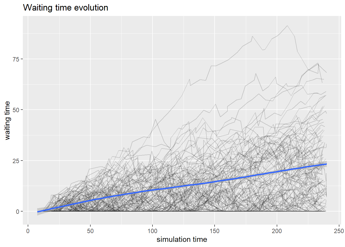

Each black line represents a single simulation and the blue line gives an overall representation of the simulation. We can see that the waiting time seems to be linearly increasing with time.