3.4 Notable Continuous Distribution
As in the discrete case, there are some types of continuous random variables that are used frequently and therefore are given a name and their proprieties are well-studied.
3.4.1 Uniform Distribution
The first, and simplest, continuous random variable we study is the so-called (continuous) uniform distribution. We say that a random variable \(X\) is uniformly distributed on the interval \([a,b]\) if its pdf is \[ f(x)=\left\{ \begin{array}{ll} \frac{1}{b-a}, & a\leq x \leq b\\ 0, & \mbox{otherwise} \end{array} \right. \] This is plotted in Figure 3.9 for choices of parameters \(a=2\) and \(b=6\)
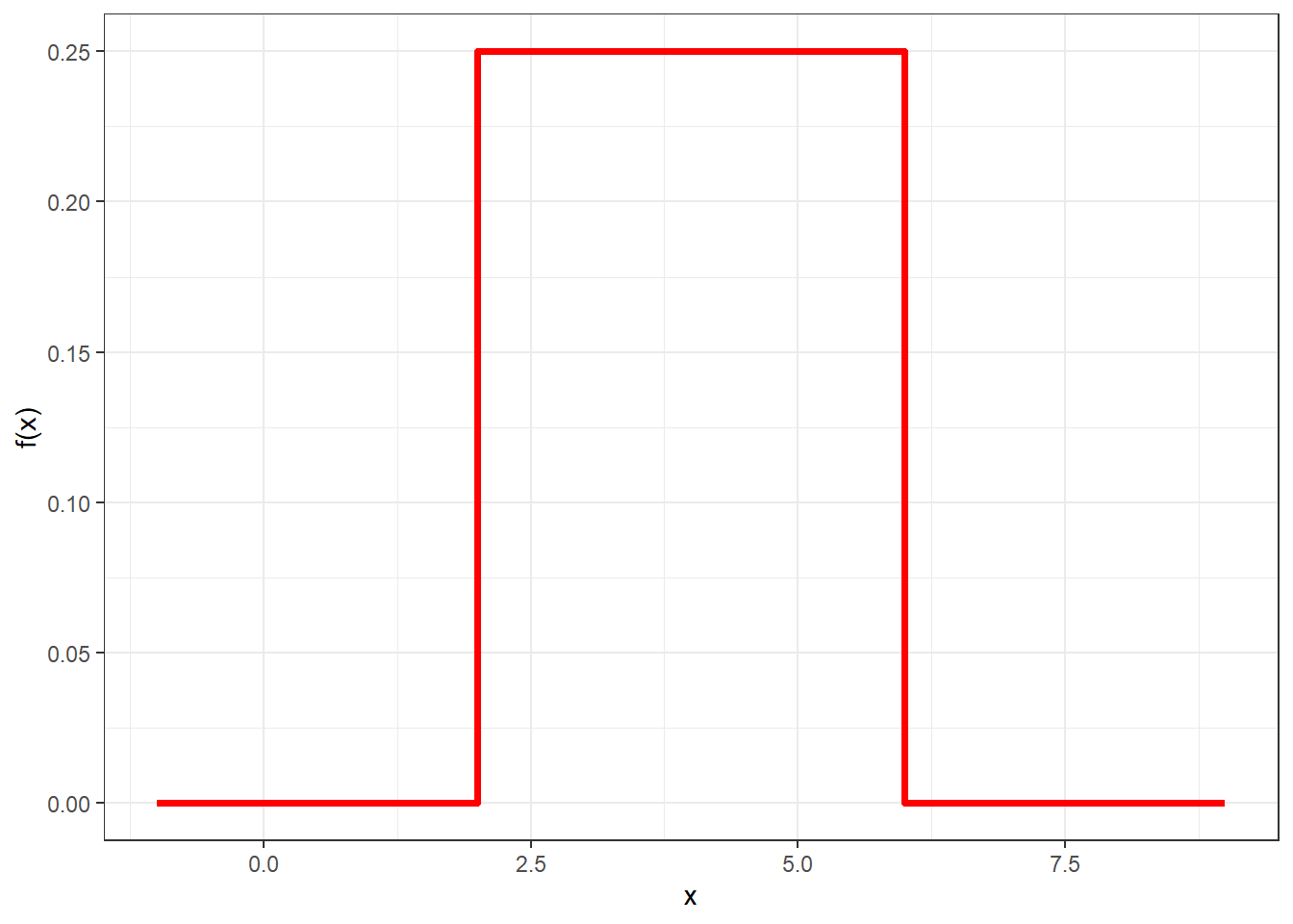
Figure 3.9: Probability density function for a uniform random variable with parameters a = 2 and b = 6
By looking at the pdf we see that it is a flat, constant line between the values \(a\) and \(b\). This implies that the probability that \(X\) takes values between two values \(x_0\) and \(x_1\) only dependens on the length of the interval \((x_0,x_1)\).
Its cdf can be derived as \[ F(x)=\left\{ \begin{array}{ll} 0, & x<a\\ \frac{x-a}{b-a}, & a\leq x \leq b\\ 1, & x>b \end{array} \right. \] and this is plotted in Figure 3.10.
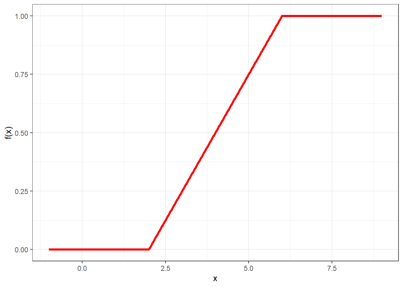
Figure 3.10: Cumulative distribution function for a uniform random variable with parameters a = 2 and b = 6
The mean and variance of a uniform can be derived as \[ E(X)=\frac{a+b}{2}, \hspace{1cm} V(X)=\frac{(b-a)^2}{12}. \] So the mean is equal to the middle point of the interval \((a,b)\).
The uniform distribution will be fundamental in simulation. We will see that the starting point to simulate random numbers from any distribution will require the simulation of random numbers uniformly distributed between 0 and 1.
R provides an implementation of the uniform random variable with the functions dunif and punif whose details are as follows:
the first argument is the value at which to compute the function;
the second argument,
min, is the parameter \(a\), by default equal to zero;the third argument,
max, is the parameter \(b\), by default equal to one.
So for instance
dunif(5, min = 2, max = 6)## [1] 0.25computes the pdf at the point 5 of a uniform random variable with parameters \(a=2\) and \(b=6\).
Conversely,
punif(0.5)## [1] 0.5computes the cdf at the point 0.5 of a uniform random variable with parameters \(a=0\) and \(b=1\).
3.4.2 Exponential Distribution
The second class of continuous random variables we will study are the so-called exponential random variables. We have actually already seen such a random variable in the donut shop example. More generally, we say that a continuous random variable \(X\) is exponential with parameter \(\lambda>0\) if its pdf is \[ f(x) = \left\{ \begin{array}{ll} \lambda e^{-\lambda x}, & x\geq 0\\ 0, & \mbox{otherwise} \end{array} \right. \]
Figure 3.11 reports the pdf of exponential random variables for various choices of the parameter \(\lambda\).
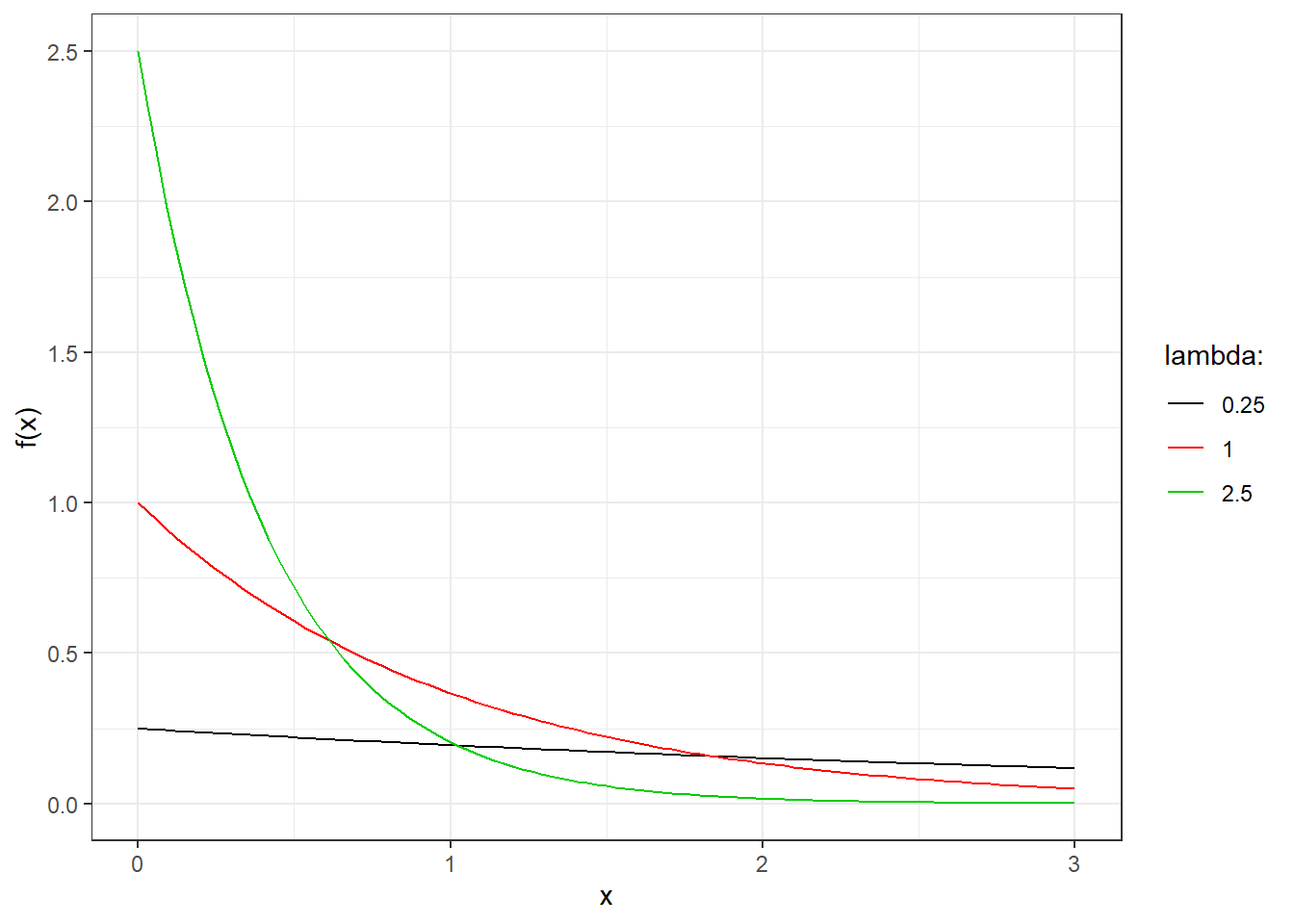
Figure 3.11: Probability density function for exponential random variables
Exponential random variables are very often used in dynamic simulations since they are very often used to model interarrival times in process: for instance the time between arrivals of customers at the donut shop.
Its cdf can be derived as \[ F(x)=\left\{ \begin{array}{ll} 0, & x <0\\ 1-e^{-\lambda x}, & x\geq 0 \end{array} \right. \] and is reported in Figure 3.12 for the same choices of parameters.
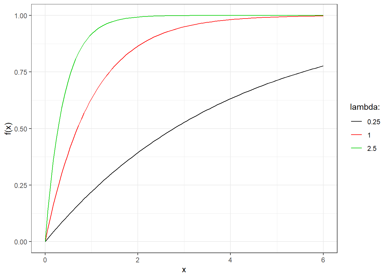
Figure 3.12: Cumulative distribution function for exponential random variables
The mean and the variance of exponential random variables can be computed as
\[ E(X)=\frac{1}{\lambda}, \hspace{1cm} V(X)=\frac{1}{\lambda^2} \]
R provides an implementation of the uniform random variable with the functions dexp and pexp whose details are as follows:
the first argument is the value at which to compute the function;
the second argument,
rate, is the parameter \(\lambda\), by default equal to one;
So for instance
dexp(2, rate = 3)## [1] 0.007436257computes the pdf at the point 2 of an exponential random variable with parameter \(\lambda =3\).
Conversely
pexp(4)## [1] 0.9816844computes the cdf at the point 4 of an exponential random variable with parameter \(\lambda =1\).
3.4.3 Normal Distribution
The last class of continuous random variables we consider is the so-called Normal or Gaussian random variable. They are the most used and well-known random variable in statistics and we will see why this is the case.
A continuous random variable \(X\) is said to have a Normal distribution with mean \(\mu\) and variance \(\sigma^2\) if its pdf is \[ f(x) = \frac{1}{\sqrt{2\pi\sigma^2}}\exp\left(-\frac{1}{2}\frac{(x-\mu)^2}{\sigma^2}\right). \] Recall that \[ E(X)=\mu, \hspace{1cm} V(X)=\sigma^2, \] and so the parameters have a straightforward interpretation in terms of mean and variance.
Figure 3.13 shows the form of the pdf of the Normal distribution for various choices of the parameters. On the left we have Normal pdfs for \(\sigma^2=1\) and various choices of \(\mu\): we can see that \(\mu\) shifts the plot on the x-axis. On the right we have Normal pdfs for \(\mu=1\) and various choices of \(\sigma^2\): we can see that all distributions are centered around the same value while they have a different spread/variability.
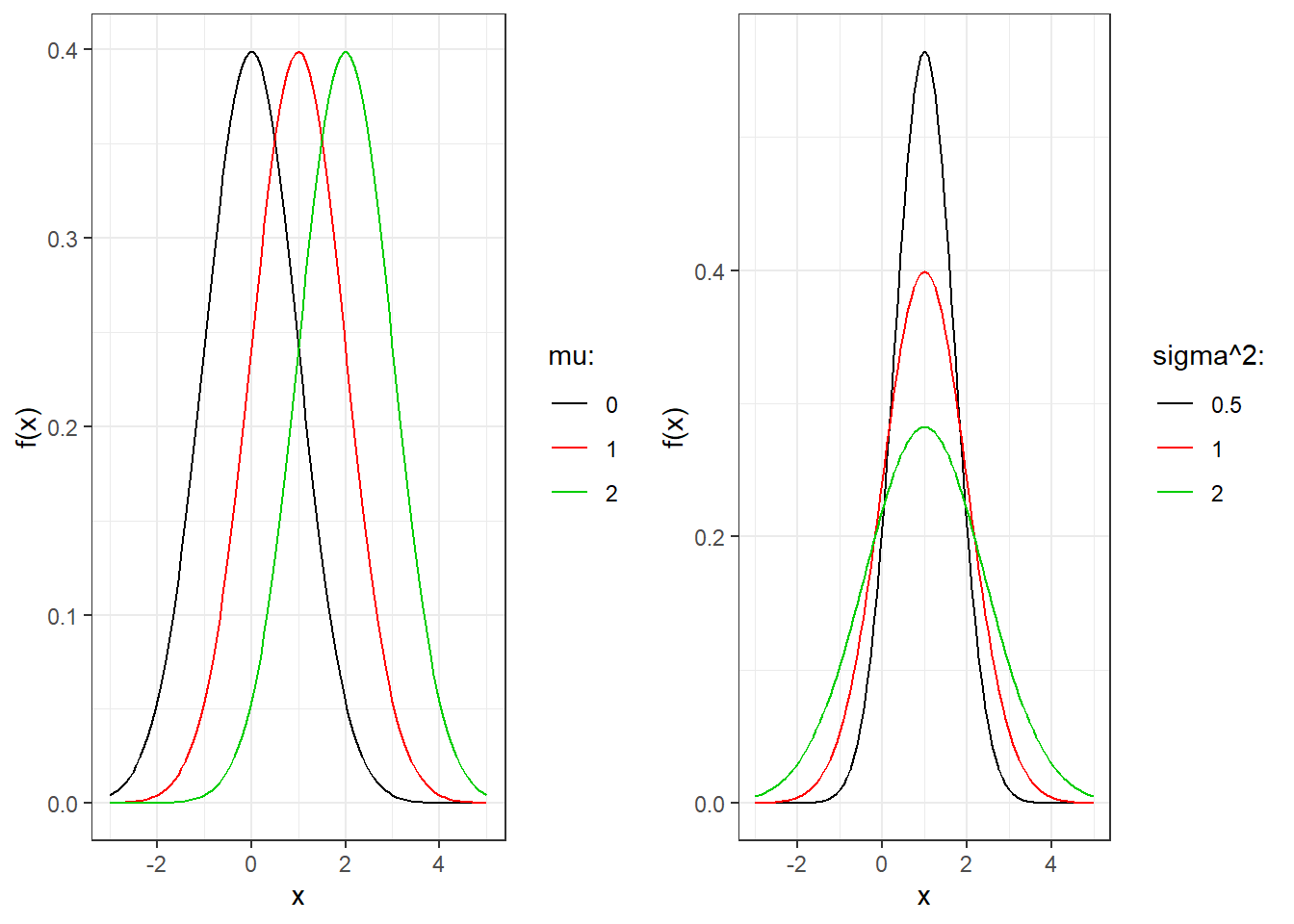
Figure 3.13: Probability density function for normal random variables
The form of the Normal pdf is the well-known so-called bell-shaped function. We can notice some properties:
it is symmetric around the mean: the function on the left-hand side and on the right-hand side of the mean is mirrored. This implies that the median is equal to the mean ;
the maximum value of the pdf occurs at the mean. This implies that the mode is equal to the mean (and therefore also the median).
The cdf of the Normal random variable with parameters \(\mu\) and \(\sigma^2\) is \[ F(x) = P(X\leq x)=\int_{-\infty}^{+\infty}\frac{1}{\sqrt{2\pi\sigma^2}}\exp\left(-\frac{1}{2}\frac{(x-\mu)^2}{\sigma^2}\right)dx \]
The cdf of the Normal for various choices of parameters is reported in Figure 3.14.
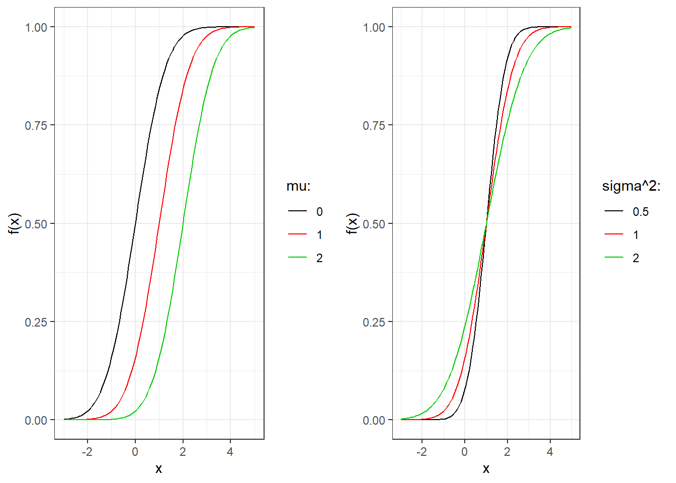
Figure 3.14: Cumulative distribution function for normal random variables
Unfortunately it is not possible to solve such an integral (as for example for the Uniform and the Exponential), and in general it is approximated using some numerical techniques. This is surprising considering that the Normal distribution is so widely used!!!
However, notice that we would need to compute such an approximation for every possible value of \((\mu,\sigma^2)\), depending on the distribution we want to use. This is unfeasible to do in practice.
There is a trick here, that you must have used multiple times already. We can transform a Normal \(X\) with parameters \(\mu\) and \(\sigma^2\) to the so-called standard Normal random variable \(Z\), and viceversa, using the relationship: \[\begin{equation} \tag{3.1} Z = \frac{X-\mu}{\sigma}, \hspace{1cm} X= \mu + \sigma Z. \end{equation}\] It can be shown that \(Z\) is a Normal random variable with parameter \(\mu=0\) and \(\sigma^2=1\).
The values of the cdf of the standard Normal random variable then need to be computed only once since \(\mu\) and \(\sigma^2\) are fixed. You have seen these numbers many many times in what are usually called the tables of the Normal distribution.
As a matter of fact you have also computed many times the cdf of a generic Normal random variable. First you computed \(Z\) using equation (3.1) and then looked at the Normal tables to derive that number.
Let’s give some details about the standard Normal. Its pdf is \[ \phi(z)=\frac{1}{\sqrt{2\pi}}\exp\left(-z^2/2\right). \] It can be seen that it is the same as the one of the Normal by setting \(\mu=0\) and \(\sigma^2=1\). Such a function is so important that it is given its own symbol \(\phi\).
The cdf is \[ \Phi(z)=\int_{-\infty}^z\frac{1}{\sqrt{2\pi}}\exp\left(-x^2/2\right)dx \] Again this cannot be computed exactly, there is no closed-form expression. This is why you had to look at the tables instead of using a simple formula. The cdf of the standard Normal is also so important that it is given its own symbol \(\phi\).
Instead of using the tables, we can use R to tell us the values of Normal probabilities. R provides an implementation of the Normal random variable with the functions dnorm and pnorm whose details are as follows:
the first argument is the value at which to compute the function;
the second argument,
mean, is the parameter \(\mu\), by default equal to zero;the third argument,
sd, is the standard deviation, that is \(\sqrt{\sigma^2}\), by default equal to one.
So for instance
dnorm(3)## [1] 0.004431848computes the value of the standard Normal pdf at the value three.
Similarly,
pnorm(0.4,1,0.5)## [1] 0.1150697compute the value of the Normal cdf with parameters \(\mu=1\) and \(\sqrt{\sigma^2}=0.5\) at the value 0.4.