3.1 Discrete Random Variables
We start introducing discrete random variables. Here we will not enter in all the mathematical details and some concepts will be introduced only intuitively. However, some mathematical details will be given for some concepts.
In order to introduce discrete random variables, let’s inspect each of the words:
variable: this means that there is some process that takes some value. It is a synonym of function as you have studied in other mathematics classes.
random: this means that the variable takes values according to some probability distribution.
discrete: this refers to the possible values that the variable can take. In this case it is a countable (possibly infinite) set of values.
In general we denote a random variable as \(X\) and its possible values as \(\mathbb{X}=\{x_1,x_2,x_3,\dots\}\). The set \(\mathbb{X}\) is called the sample space of \(X\). In real-life we do not know which value in the set \(\mathbb{X}\) the random variable will take.
Let’s consider some examples.
The number of donuts sold in a day in a shop is a discrete random variable which can take values \(\{0,1,2,3,\dots\}\), that is the non-negative integers. In this case the number of possible values is infinite.
The outcome of a COVID-19 test can be either positive or negative but in advance we do not know which one. So this can be denoted as a discrete random variable taking values in \(\{negative,positive\}\). It is customary to denote the elements of the sample space \(\mathbb{X}\) as numbers. For instance, we could let \(negative = 0\) and \(positive = 1\) and the sample space would be \(\mathbb{X}=\{0,1\}\).
The number shown on the face of a dice once thrown is a discrete random variable taking values in \(\mathbb{X}=\{1,2,3,4,5,6\}\).
3.1.1 Probability Mass Function
The outcome of a discrete random variable is in general unknown, but we want to associate to each outcome, that is to each element of \(\mathbb{X}\), a number describing its likelihood. Such a number is called a probability and it is in general denoted as \(P\).
The probability mass function (or pmf) of a random variable \(X\) with sample space \(\mathbb{X}\) is defined as \[ p(x)=P(X=x), \hspace{1cm} \mbox{for all } x\in\mathbb{X} \] So for any outcome \(x\in\mathbb{X}\) the pmf describes the likelihood of that outcome happening.
Recall that pmfs must obey two conditions:
\(p(x)\geq 0\) for all \(x\in\mathbb{X}\);
\(\sum_{x\in\mathbb{X}}p(x)=1\).
So the pmf associated to each outcome is a non-negative number such that the sum of all these numbers is equal to one.
Let’s consider an example at this stage. Suppose a biased dice is thrown such that the numbers 3 and 6 are twice as likely to appear than the other numbers. A pmf describing such a situation is the following:
| \(x\) | 1 | 2 | 3 | 4 | 5 | 6 |
|---|---|---|---|---|---|---|
| \(p(x)\) | 1/8 | 1/8 | 2/8 | 1/8 | 1/8 | 2/8 |
It is apparent that all numbers \(p(x)\) are non-negative and that their sum is equal to 1: so \(p(x)\) is a pmf. Figure 3.1 gives a graphical visualization of such a pmf.
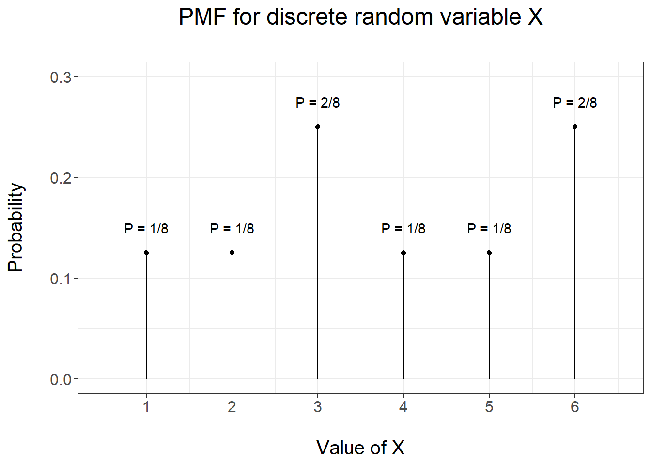
Figure 3.1: PMF for the biased dice example
3.1.2 Cumulative Distribution Function
Whilst you should have been already familiar with the concept of pmf, the next concept may appear to be new. However, you have actually used it multiple times when computing Normal probabilities with the tables.
We now define what is usually called the cumulative distribution function (or cdf) of a random variable \(X\). The cdf of \(X\) at the point \(x\in\mathbb{X}\) is \[ F(x) = P(X \leq x) = \sum_{y \leq x} p(y) \] that is the probability that \(X\) is less or equal to \(x\) or equally the sum of the pmf of \(X\) for all values less than \(x\).
Let’s consider the dice example to illustrate the idea of cdf and consider the following values \(x\):
\(x=0\): we compute \(F(0) = P(X\leq 0 )= 0\) since \(X\) cannot take any values less or equal than zero;
\(x= 0.9\): we compute \(F(0.9)= P(X\leq 0.9) = 0\) using the same reasoning as before;
\(x = 1\): we compute \(F(1)= P(X\leq 1) = P(X=1) = 1/8\) since \(X\) can take the value 1 with probability 1/8;
\(x = 1.5\): we compute \(F(1.5) = P(X\leq 1.5) = P(X=1) = 1/8\) using the same reasoning as before;
\(x = 3.2\): we compute \(F(3.2)=P(X\leq 3.2)=P(X=1)+ P(X=2) + P(X=3)=1/8 + 1/8 + 2/8 = 0.5\) since \(X\) can take the values 1, 2 and 3 which are less than 3.2;
We can compute in a similar way the cdf for any value \(x\). A graphical visualization of the resulting CDF is given in Figure 3.2.
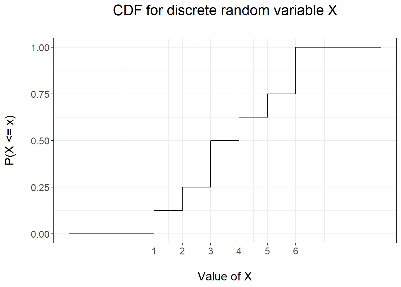
Figure 3.2: CDF for the biased dice example
The plot highlights some properties of CDFs which can proved hold in general for any discrete CDF:
it is a step function which is also non-decreasing;
on the left-hand-side it takes the value 0;
on the right-hand-side it takes the value 1.
3.1.3 Summaries
The pmf and the cdf fully characterize a discrete random variable \(X\). Often however we want to compress that information into a single number which still retains some aspect of the distribution of \(X\).
The expectation or mean of a random variable \(X\) denoted as \(E(X)\) is defined as \[ E(X)=\sum_{x\in\mathbb{X}}xp(x) \] The expectation can be interpreted as the mean value of a large number of observations from the random variable \(X\). Consider again the example of the biased dice. The expectation is \[ E(X)=1\cdot1/8 + 2\cdot1/8 + 3\cdot 2/8 + 4\cdot 1/8 + 5\cdot 1/8 + 6\cdot 2/8 = 3.75 \] So if we were to throw the dice a large number of time, we would expect the average of the number shown to be 3.75.
The median of the random variable \(X\) denoted as \(m(X)\) is defined as the value \(x\) such that \(P(X\leq x)\) is larger or equal to 0.5 and \(P(X\geq x)\) is larger or equal to 0.5. It is defined as the middle value of the distribution. For the dice example the median is the value 3: indeed \(P(X\leq 3 ) = P(X=1)+P(X=2)+P(X=3)=0.5 \geq 0.5\) and \(P(X\geq 3) = P(X=3) + P(X=4) + P(X=5) + P(X=6) = 0.75 \geq 0.5\).
The mode of the random variable \(X\) is the value \(x\) such that \(p(x)\) is largest: it is the value of the random variable which is expected to happen most frequently. Notice that the mode may not be unique: in that case we say that the distribution of \(X\) is bimodal. The example of the biased dice as an instance of a bimodal distribution: the values 3 and 6 are the equally likely and they have the largest pmf.
The above three summaries are measures of centrality: they describe the central tendency of \(X\). Next we consider measures of variability: such measures will quantify the spread or the variation of the possible values of \(X\) around the mean.
The variance of the discrete random variable \(X\) is the expectation of the squared difference between the random variable and its mean. Formally it is defined as \[ V(X)=E((X-E(X))^2)=\sum_{x\in\mathbb{X}}(x-E(X))^2p(x) \] In general we will not compute variance by hand. The following R code computes the variance of the random variable associated to the biased dice.
x <- 1:6  # outcomes of X
px <- c(1/8,1/8,2/8,1/8,1/8,2/8)  # pmf of X
Ex <- sum(x*px)  # Expectation of X
Vx <- sum((x-Ex)^2*px)  # Variance of X
Vx
## [1] 2.9375The standard deviation of the discrete random variable \(X\) is the square root of \(V(X)\).