3.3 Continuous Random Variables
Our attention now turns to continuous random variables. These are in general more technical and less intuitive than discrete ones. You should not worry about all the technical details, since these are in general not important, and focus on the interpretation.
A continuous random variable \(X\) is a random variable whose sample space \(\mathbb{X}\) is an interval or a collection of intervals. In general \(\mathbb{X}\) may coincide with the set of real numbers \(\mathbb{R}\) or some subset of it. Examples of continuous random variables:
the pressure of a tire of a car: it can be any positive real number;
the current temperature in the city of Madrid: it can be any real number;
the height of the students of Simulation and Modeling to understand change: it can be any real number.
Whilst for discrete random variables we considered summations over the elements of \(\mathbb{X}\), i.e. \(\sum_{x\in\mathbb{X}}\), for continuous random variables we need to consider integrals over appropriate intervals.
You should be more or less familiar with these from previous studies of calculus. But let’s give an example. Consider the function \(f(x)=x^2\) computing the squared of a number \(x\). Suppose we are interested in this function between the values -1 and 1, which is plotted by the red line in Figure 3.6. Consider the so-called integral \(\int_{-1}^{1}x^2dx\): this coincides with the area delimited by the function and the x-axis. In Figure 3.6 the blue area is therefore equal to \(\int_{-1}^{1}x^2dx\).
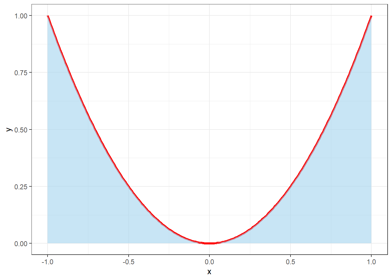
Figure 3.6: Plot of the squared function and the area under its curve
We will not be interested in computing integrals ourselves, so if you do not know/remember how to do it, there is no problem!
3.3.1 Probability Density Function
Discrete random variable are easy to work with in the sense that there exists a function, that we called probability mass function, such that \(p(x)=P(X=x)\), that is the value of that function in the point \(x\) is exactly the probability that \(X=x\).
Therefore we may wonder if this is true for a continuous random variable too. Sadly, the answer is no and probabilities for continuous random variables are defined in a slightly more involved way.
Let \(X\) be a continuous random variable with sample space \(\mathbb{X}\). The probability that \(X\) takes values in the interval \([a,b]\) is given by \[ P(a\leq X \leq b) = \int_{a}^bf(x)dx \] where \(f(x)\) is called the probability density function (pdf in short). Pdfs, just like pmfs must obey two conditions:
\(f(x)\geq 0\) for all \(x\in\mathbb{X}\);
\(\int_{x\in\mathbb{X}}f(x)dx=1\).
So in the discrete case the pmf is defined exactly as the probability. In the continuous case the pdf is the function such that its integral is the probability that random variable takes values in a specific interval.
As a consequence of this definition notice that for any specific value \(x_0\in\mathbb{X}\), \(P(X=x_0)=0\) since \[ \int_{x_0}^{x_0}f(x)dx = 0. \]
Let’s consider an example. The waiting time of customers of a donuts shop is believed to be random and to follow a random variable whose pdf is \[ f(x) = \left\{ \begin{array}{ll} \frac{1}{4}e^{-x/4}, & x\geq 0\\ 0, & \mbox{otherwise} \end{array} \right. \]
The pdf is drawn in Figure 3.7 by the red line. One can see that \(f(x)\geq 0\) for all \(x\geq 0\) and one could also compute that it integrates to one.
Therefore the probability that the waiting time is between any two values \((a,b)\) can be computed as \[ \int_a^b\frac{1}{4}e^{-x/4}dx. \] In particular if we were interested in the probability that the waiting time is between two and five minutes, corresponding to the shaded area in Figure 3.7, we could compute it as \[ P(2<X<5)=\int_2^5f(x)dx=\int_{2}^5\frac{1}{4}e^{-x/4}dx= 0.32 \]
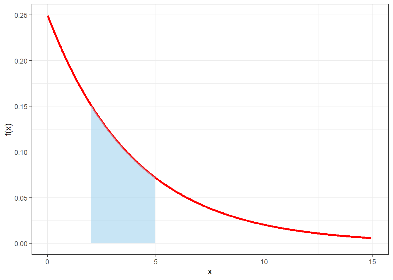
Figure 3.7: Probability density function for the waiting time in the donut shop example
Notice that since \(P(X=x_0)=0\) for any \(x_0\in\mathbb{X}\), we also have that \[ P(a\leq X \leq b)=P(a < X \leq b) = P(a\leq X < b) = P(a<X<b). \]
3.3.2 Cumulative Distribution Function
For a continuous random variable \(X\) the cumulative distribution function (cdf) is equally defined as \[ F(x) = P(X \leq x), \] where now \[ P(X \leq x) = P(X < x) = \int_{-\infty}^xf(t)dt. \] so the summation is substituted by an integral.
Let’s consider again the donut shop example as an illustration. The cdf is defined as \[ F(x)=\int_{-\infty}^xf(t)dt = \int_{-\infty}^x\frac{1}{4}e^{-x/4}. \] This integral can be solved and \(F(x)\) can be calculated as \[ F(x)= 1- e^{-x/4}, \] which is plotted in Figure 3.8.
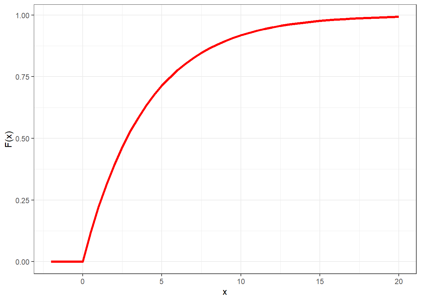
Figure 3.8: Cumulative distribution function for the waiting time at the donut shop
We can notice that the cdf has similar properties as in the discrete case: it is non-decreasing, on the left-hand side is zero and on the right-hand side tends to zero.
In the continuous case, one can prove that cdfs and pdfs are related as \[ f(x)=\frac{d}{dx}F(x). \]
3.3.3 Summaries
Just as for discrete random variables, we may want to summarize some features of a continuous random variable into a unique number. The same set of summaries exists for continuous random variables, which are almost exactly defined as in the discrete case (integrals are used instead of summations).
mean: the mean of a continuous random variable \(X\) is defined as \[ E(X) = \int_{-\infty}^{+\infty}xf(x)dx \]
median: the median of a continuous random variable \(X\) is defined as the value \(x\) such that \(P(X\leq x) = 0.5\) or equally \(F(x)=0.5\).
mode: the mode of a continuous random variable \(X\) is defined the value \(x\) such that \(f(x)\) is largest.
variance: the variance of a continuous random variable \(X\) is defined as \[ V(X)=\int_{-\infty}^{+\infty}(x-E(X))^2f(x)dx \]
standard deviation: the standard deviation of a continuous random variable \(X\) is defined as \(\sqrt{V(X)}\).