7.4 Measures of Performance
There are various measures that one can use to assess the quality of a queuing system. These are:
\(L\): the average number of customers in the system;
\(L_Q\): the average number of customers in the system;
\(w\): the average time spent in the system;
\(w_Q\): the average time spent in the queue;
\(\rho\): the server utilization; the proportion of time that a server is busy.
The term system refers to the waiting line plus the service mechanism, whilst the term queue refers to the waiting line alone.
7.4.1 Average Number of Customers in the System \(L\)
Consider a queuing system over a period of time \(T\) and let \(L(t)\) denote the number of customers in the system at time \(t\). Let \(T_i\) be the total time in \([0,T]\) in which the system contained exactly \(i\) customers. In general \(\sum_{i=0}^{\infty}T_i = T\). The average number of customers in the system is estimated by \[ \hat{L}=\frac{1}{T}\sum_{i=0}^\infty iT_i=\sum_{i=0}^\infty i \frac{T_i}{T}. \] Notice that \(T_i/T\) is the proportion of time the system contains exactly \(i\) customers.
Let’s consider an example. Figure 7.1 gives a simulation of a queue in an interval of 20 time units. It can be seen that \(T_0= 3\), \(T_1 = 11\), \(T_2 = 5\) and \(T_3 =1\), and therefore \(\hat{L}= (0\cdot 3 + 1\cdot 11 + 2\cdot 5 + 3\cdot 1)/20 = 24/20 = 1.2\) customers.
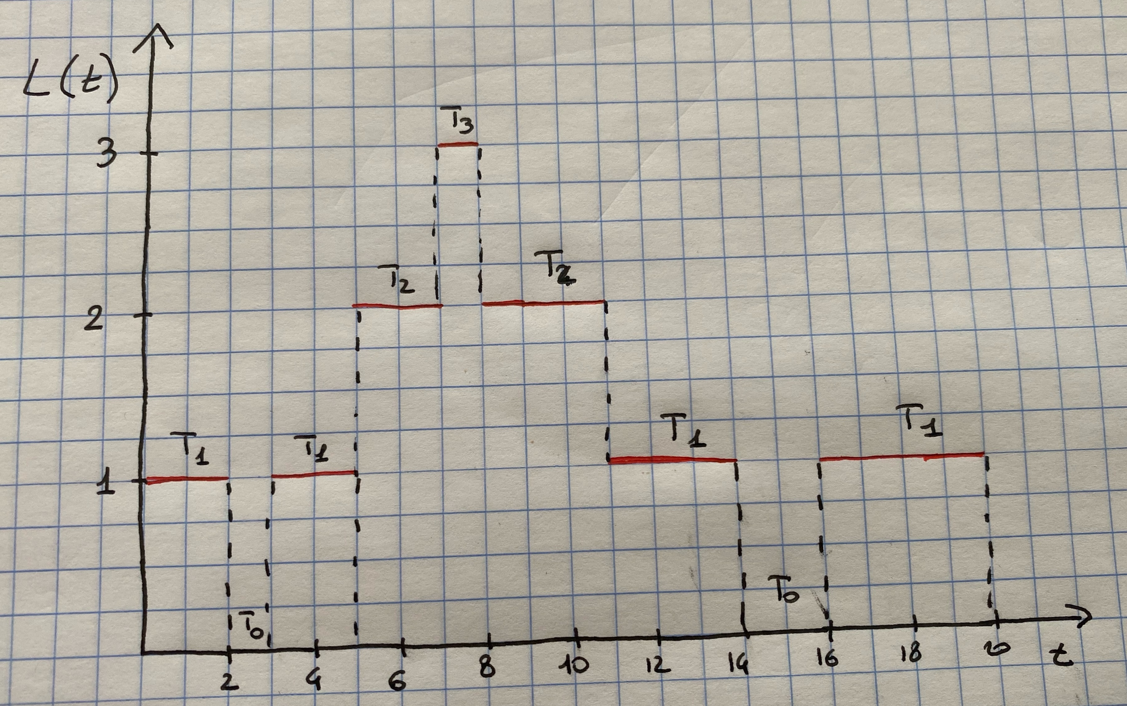
Figure 7.1: Number in system, L(t), at time t.
By looking at Figure 7.1 it can be seen that the total area under the function \(L(t)\) can be decomposed into rectangles of length \(T_i\) and height \(i\), thus having area \(iT_i\). It follows that the total area is given by \[ \sum_{i=0}^{\infty}iT_i = \int_0^TL(t)dt \] and therefore \[ \hat{L}= \frac{1}{T}\sum_{i=0}^{\infty}iT_i=\frac{1}{T}\int_{0}^TL(t)dt \]
Many queuing systems exhibit some kind of long-run stability in terms of their average performance. For such systems, as time \(T\) gets large, the observed average number of customers in the system \(\hat{L}\) approaches a limiting value, say \(L\), which is called the long-run average number in system. With probability 1 we have that \[ \hat{L}=\frac{1}{T}\int_{0}^TL(t)dt \rightarrow L \mbox{ as } T \rightarrow \infty \] If a simulation run length \(T\) is sufficiently long, the estimator \(\hat{L}\) becomes arbitrarily close to \(L\).
The above equations can be applied to any subsystem of a queuing system. If \(L_Q(t)\) denotes the number of customers waiting in queue, and \(T_i^Q\) denotes the total time in \([0,T]\) in which exactly \(i\) customers are waiting in queue, then \[ \hat{L}_Q=\frac{1}{T}\sum_{i=0}^{\infty}iT_i^Q=\int_0^TL_Q(t)dt \rightarrow L_Q \mbox{ as } T \rightarrow \infty \]
7.4.2 Average Time Spent in System per Customer \(w\)
If we simulate a queuing system for some period of time, say \(T\), then we can record the time that each customer spends in the system during \([0,T]\), say \(W_1,W_2,\dots,W_N\) where \(N\) is the number of arrivals in \([0,T]\). The average time spent in system per customer, called the average system time, is given by \[ \hat{w} = \frac{1}{N}\sum_{i=1}^N W_i \] For stable systems, as \(N\rightarrow \infty\) \[ \hat{w} \rightarrow w \] with probability 1, where \(w\) is called the long-run average system time.
If the system under consideration is the queue alone, we can re-write the above equations as \[ \hat{w}_Q=\frac{1}{N}\sum_{i=1}^NW_i^Q \rightarrow w_Q \mbox{ as } N \rightarrow \infty \] where \(W_i^Q\) is the total time customer \(i\) spends waiting in queue, \(\hat{w}_Q\) is the observed average time spend in queue (or delay) and \(w_Q\) is the long-run average delay per customer.
Consider the system in Figure 7.1. It can be seen that there are 5 customers who waited \(W_1 =2\), \(W_2 = 5\), \(W_3 = 6\), \(W_4 = 7\) and \(W_5 = 4\) and therefore \[ \hat{w}=\frac{2+5 +6 + 7 + 4}{5}= 4.8 \mbox{ time units} \] Thus on average these customers spent 4.8 time units in the system. As for the time spent in the queue, it can be computed as \(W_1^Q=0\), \(W_2^Q = 0\), \(W_3^Q=3\), \(W_4^Q = 4\) and \(W_5^Q = 0\), thus: \[ \hat{w}_Q=\frac{0 + 0 + 3 + 4 +0}{5}= 1.4 \mbox{ time units.} \]
7.4.3 Little’s Law
For the example in Figure 7.1 there were \(N=5\) arrivals in \(T=20\) time units, and thus the observed arrival rate was \(\hat{\lambda}= N/T=1/4\) customer per time unit. Recall that \(\hat{L}=1.2\) and \(\hat{w}=4.8\). Hence it follows that \[ \hat{L}=\hat{\lambda}\hat{w}, \] since \(1.2 = \frac{1}{4}4.8\).
This relationship is not coincidental: it holds for almost all queuing systems. Allowing \(T\rightarrow \infty\) and \(N\rightarrow \infty\), the above expression becomes \[ L=\lambda w, \] where \(\hat{\lambda}\rightarrow \lambda\) and \(\lambda\) is the long-run average arrival rate. This equality is usually called Little’s law. It says that the average number of customers in the system is equal to the average number of arrivals per time unit times the average time spent in the system. For Figure 7.1 there is one arrival every 4 minutes (on average) and each arrival spends 4.6 minutes in the system (on average), so at an arbitrary point in time there will be \((1/4)(4.9)=1.2\) customers present (on average).
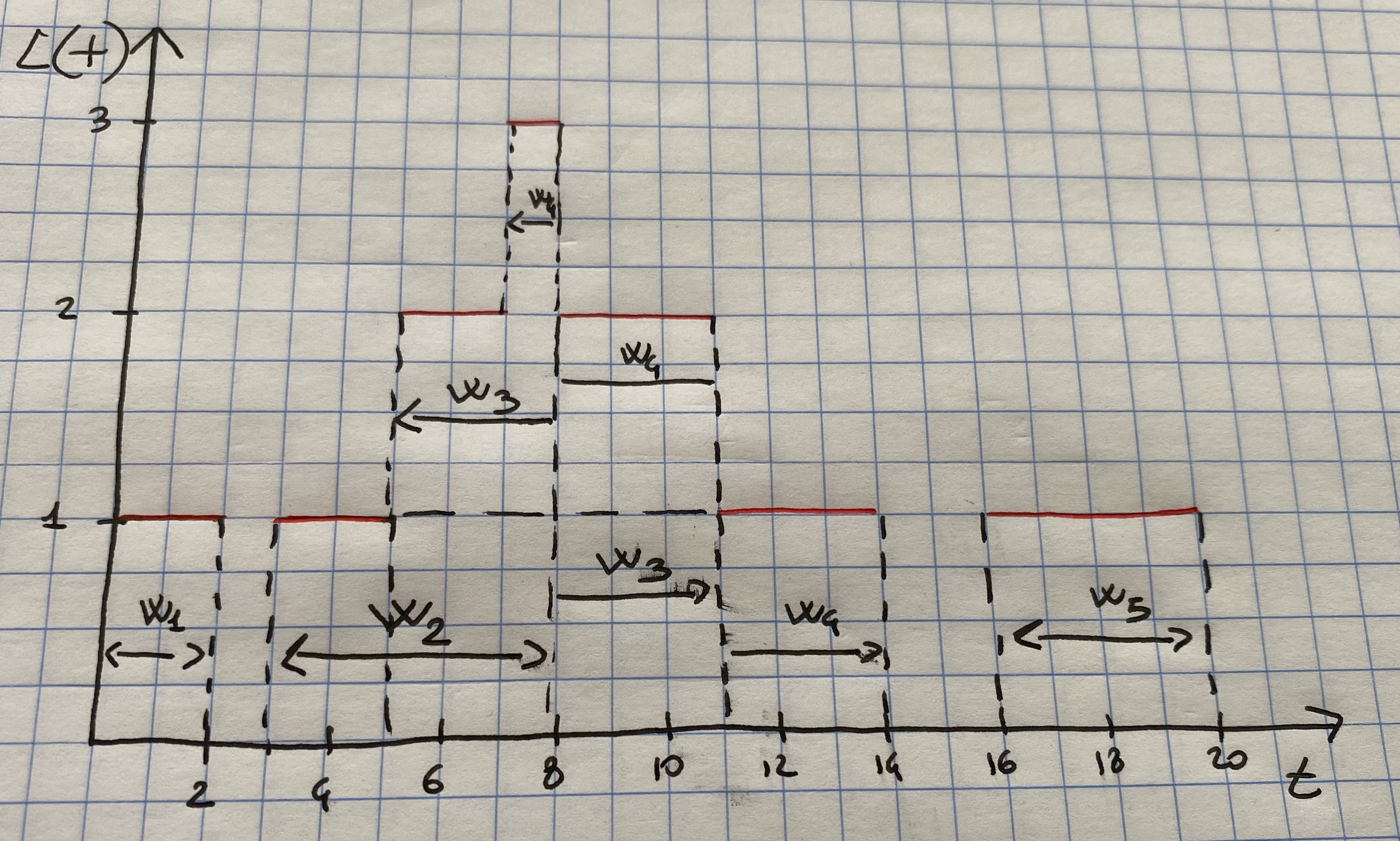
Figure 7.2: System times W_i for the example system.
Little’s law can also be derived reconsidering Figure 7.1 as follows. Figure ?? shows the exact same system history, but reporting the waiting time of each customer in the system, \(W_i\). Again we can see that the area under the function \(L(t)\) can be decomposed into rectangles of height 1 and length \(W_i\), for each \(i=1,2,\dots,N\). Therefore \[ \sum_{i=1}^NW_i=\int_{0}^TL(t)dt \] Therefore, by using that \(\hat{\lambda}=N/T\) we have that \[ \hat{L}=\frac{1}{T}\int_{0}^TL(t)dt=\frac{1}{T}\sum_{i=1}^NW_i=\frac{N}{T}\frac{1}{N}\sum_{i=1}^NW_i=\hat\lambda\hat{w}, \] which is indeed Little’s law!
7.4.4 Server Utilization
Server utilization is defined as the proportion of time that a server is busy. Observed served utilization, denoted by \(\hat{\rho}\), is defined over a specified time interval \([0,T]\). Long-run server utilization is denoted by \(\rho\). For systems that exhibit long-run stability, \[ \hat{\rho}\rightarrow \rho \mbox{ as } T\rightarrow \infty \]
7.4.4.1 Server Utilization in G/G/1 Queues
Consider any single-server queuing system with average arrival rate \(\lambda\) customers per time unit, average service time \(E(S)=1/\mu\) time units, and infinite queue capacity and calling population. Notice that \(E(S)=1/\mu\) implies that when busy the server is working at the rate \(\mu\) customers per time unit, on average: \(\mu\) is called the service rate.
Notice that the server alone is a subsystem that can be considered as a queuing system itself. hence, Little’s law \(L=\lambda w\) can be applied to the server. For stable systems, the average arrival rate to the server, say \(\lambda_s\) must be identical to the average arrival rate to the system \(\lambda\) (certainly \(\lambda_s\leq \lambda\) since customers cannot be served faster than they arrive, but if \(\lambda_s<\lambda\) the the waiting line would tend to grow in length and so we would have an unstable system). For the server subsystem, the average system time is \(w=E(S)=1/\mu\). The actual number of customers in the server subsystem is either zero or one as shown in Figure 7.3 for the system in Figure 7.1. Hence the average number in the server subsystem \(\hat{L}_s\) is given by \[ \hat{L}_s = \frac{T-T_0}{T} \] In the example \(\hat{L}_s=17/20=\hat{\rho}\).
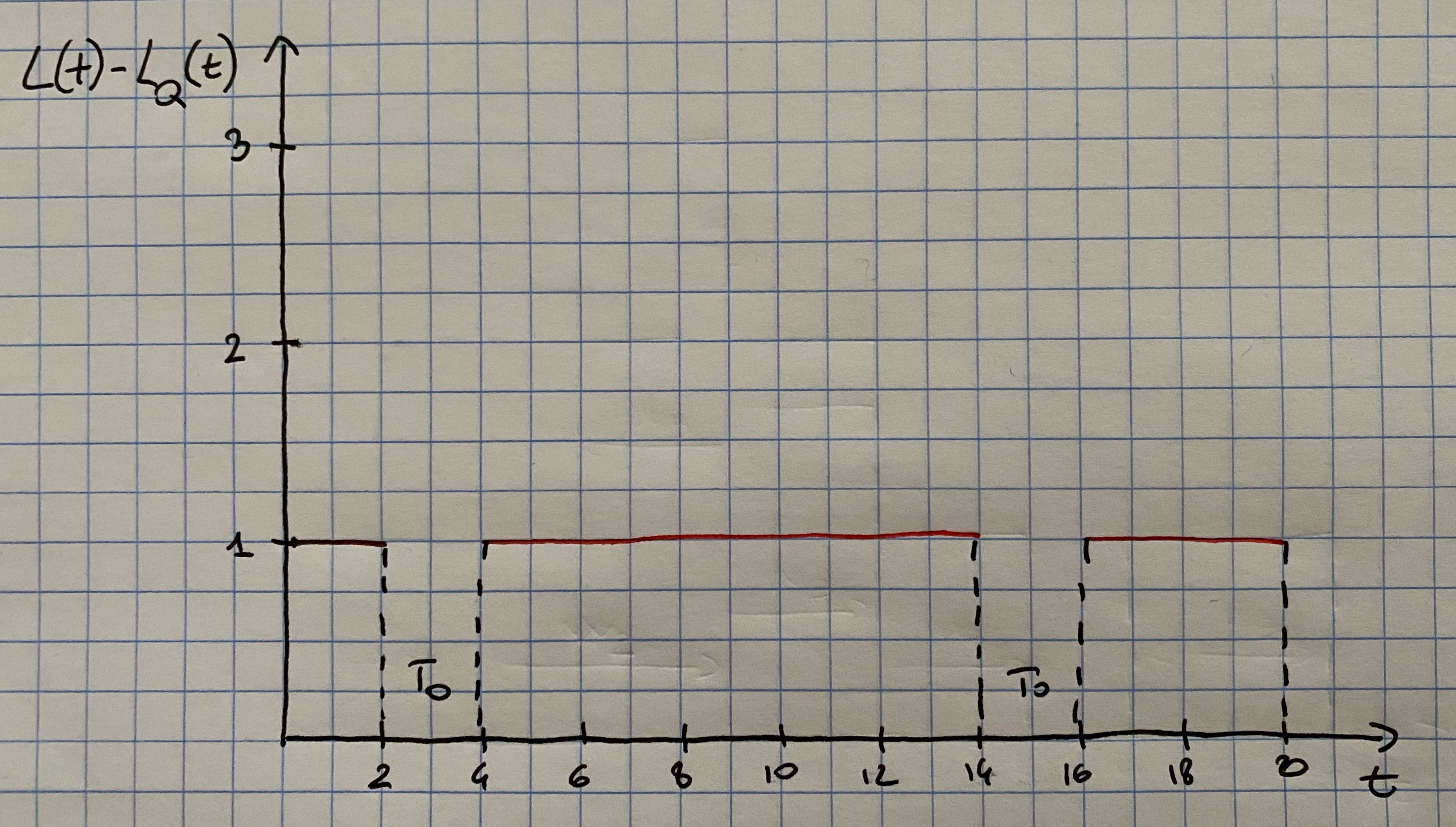
Figure 7.3: Number of customers being served at time t
In general, for a single-server queue, the average number of customers being served at an arbitrary point in time is equal to server utilization. As \(T\rightarrow \infty\), \(\hat{L}_s=\hat{\rho}\rightarrow L_s=\rho\). Combining these results into \(L=\lambda w\) for the server subsystem yields \[ \rho = \lambda E(S)=\frac{\lambda}{\mu} \] that is the long-run server utilization in a single-server queue is equal to the average arrival rate divided by the average service rate. For a single-server queue to be stable, the arrival-rate \(\lambda\) must be less then the service rate \(\mu\): \[ \lambda < \mu \] or \[ \rho =\frac{\lambda}{\mu} < 1 \] If the arrival rate is greater than the service rate \((\lambda > \mu)\) the server will eventually get further and further behind. After time, the server will always be busy, and the waiting line will tend to grow in length. For stable single-server systems long-run measures of performance such as average queue length \(L_Q\) are well defined and have a meaning. For unstable systems long-run server utilization is 1 and the long-run average queue length is infinite.
7.4.4.2 Server Utilization in G/G/c Queues
Consider now a queuing system with \(c\) identical servers in parallel. If an arriving customer finds more than one server idle, the customer chooses a server without favoring any particular server. Arrivals occur at rate \(\lambda\) from an infinite calling population and each server works at rate \(\mu\) customers per time unit.
Using a similar argument as above, one can derive that long-run average server utilization is defined by \[ \rho = \frac{\lambda}{c\mu} \] and the system is stable if \(\rho < 1\) or equivalently if \[ \lambda < c\mu. \] The average number of busy servers is \[ L_s=\frac{\lambda}{\mu}. \]
7.4.4.3 An Example
Consider a doctor who schedules patients every 10 minutes and who spends \(S_i\) minutes with the i-th patient, where \[ S_i = \left\{ \begin{array}{l} 9 \mbox{ minutes with probability } 0.9\\ 12 \mbox{ minutes with probability } 0.1 \end{array} \right. \] Thus, arrivals are deterministic (every 10 minutes) but services are stochastic with mean and variance given by \[ E(S_i)= 9\cdot 0.9 + 12\cdot 0.1 = 9.3 \mbox{ minutes} \] and \[ V(S_i)=0.9\cdot(9-9.3)^2 + 0.1\cdot(12-9.3)^2 = 0.81 \mbox{ minutes}^2 \] Here \(\rho=\lambda /\mu = 9.3/10=0.93 < 1\) and so the system is stable and the doctor will be busy 93% of the time in the long-run. In the short-run, sometimes queues will build up temporarily because of the variability of the service distribution, as shown in Figure 7.4.
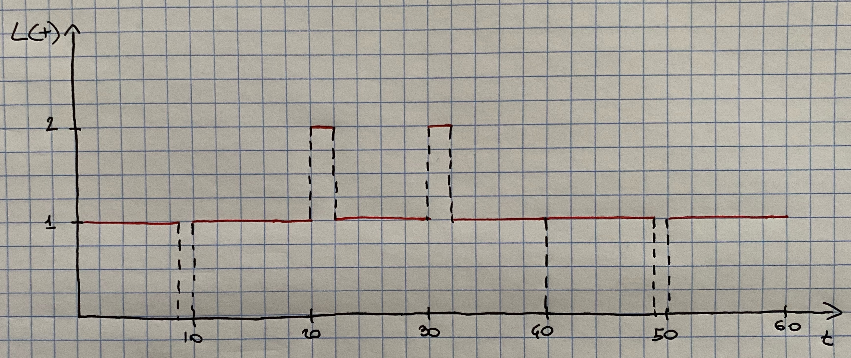
Figure 7.4: Number of patients in the doctor’s office at time t