6.5 A production process simulation
Consider a simple engineering job shop that consists of several identical machines. Each machine is able to process any job and there is a ready supply of jobs with no prospect of any shortages. Jobs are allocated to the first available machine. The time taken to complete a job is variable but is independent of the particular machine being used. The machine shop is staffed by operatives who have two tasks:
RESET machines between jobs if the cutting edges are still OK
RETOOL those machines with cutting edges that are too worn to be reset
In addition, an operator may be AWAY while attending to personal needs
The figure below shows the activity cycle diagram for the considered system. Circles (READY, STOPPED, OK, WAITING) represent states of the machines or the operatives respectively, while rectangles (RUNNING, RETOOL, RESET, AWAY) represent activities that take some (random) time to complete. Two kind of processes can be identified: shop jobs, which use machines and degrade them, and personal tasks, which take operatives AWAY for some time.
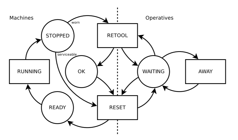
Notice that after a job is completed by a machine there may be two possible trajectories to follow:
either the machine needs only to be reset by an operator;
or it first needs to be retool and then reset by the operator.
We can implement such a situation using branch. A branch is a point in a trajectory in which one or more sub-trajectories may be followed. The branch() activity places the arrival in one of the sub-trajectories depending on some condition evaluated in a dynamical parameter called option. It is the equivalent of an if/else in programming, i.e., if the value of option is i, the i-th sub-trajectory will be executed.
Let’s implement the system. First of all, let us instantiate a new simulation environment and define the completion time for the different activities as random draws from exponential distributions. Likewise, the interarrival times for jobs and tasks are defined (NEW_JOB, NEW_TASK), and we consider a probability of 0.2 for a machine to be worn after running a job (CHECK_JOB).
set.seed(2021)
env <- simmer("Job Shop")

RUNNING <- function() rexp(1, 1)
RETOOL <- function() rexp(1, 2)
RESET <- function() rexp(1, 3)
AWAY <- function() rexp(1, 1)
CHECK_WORN <- function() runif(1) < 0.2
NEW_JOB <- function() rexp(1, 5)
NEW_TASK <- function() rexp(1, 1)
The trajectory of an incoming job starts by seizing a machine in READY state. It takes some random time for RUNNING it after which the machine’s serviceability is checked. An operative and some random time to RETOOL the machine may be needed, and either way an operative must RESET it. Finally, the trajectory releases the machine, so that it is READY again. On the other hand, personal tasks just seize operatives for some time.
task <- trajectory() %>%
  seize("operative") %>%
  timeout(AWAY) %>%
  release("operative")

job <- trajectory() %>%
  seize("machine") %>%
  timeout(RUNNING) %>%
  branch(
   CHECK_WORN, continue = TRUE,
   trajectory() %>%
   seize("operative") %>%
   timeout(RETOOL) %>%
   release("operative")) %>%
  seize("operative") %>%
  timeout(RESET) %>%
  release("operative") %>%
  release("machine")
Once the processes’ trajectories are defined, we append 10 identical machines and 5 operatives to the simulation environment, as well as two generators for jobs and tasks.
env %>%
  add_resource("machine", 10) %>%
  add_resource("operative", 5) %>%
  add_generator("job", job, NEW_JOB) %>%
  add_generator("task", task, NEW_TASK) %>%
  run(until=10)
## simmer environment: Job Shop | now: 10 | next: 10.2238404207112
## { Monitor: in memory }
## { Resource: machine | monitored: TRUE | server status: 9(10) | queue status: 0(Inf) }
## { Resource: operative | monitored: TRUE | server status: 3(5) | queue status: 0(Inf) }
## { Source: job | monitored: 1 | n_generated: 49 }
## { Source: task | monitored: 1 | n_generated: 11 }Let’s extract a history of the resource’s state to analyze the average number of machines/operatives in use as well as the average number of jobs/tasks waiting for an assignment.
aggregate(cbind(server, queue) ~ resource, get_mon_resources(env), mean)## resource server queue
## 1 machine 5.839080 0.04597701
## 2 operative 3.153153 0.30630631plot(get_mon_resources(env),"utilization")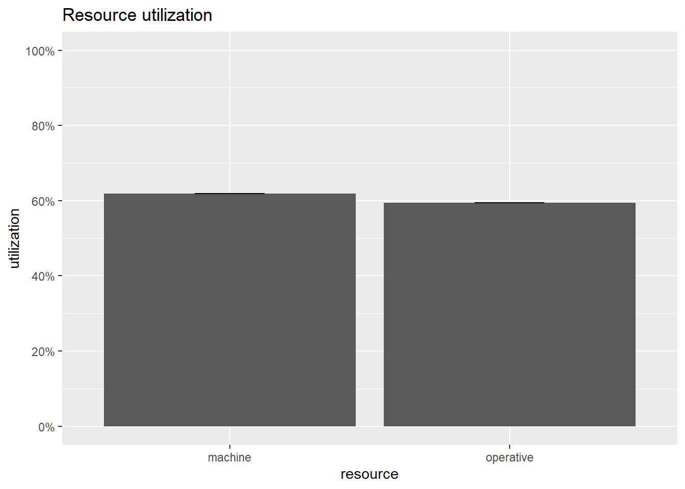
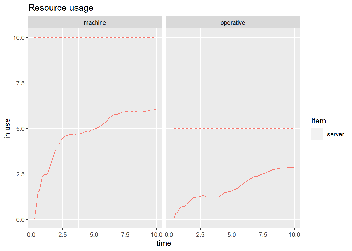
plot(get_mon_resources(env),"usage", items = "server")