Chapter 8 THE PENNSYLVANIA LUNG CANCER DATA

In this section, the dataset that will be used in the first set of examples will be introduced. This is a set of county-level lung cancer counts for 2002. The counts are stratified in ethnicity (with rather broad categories ‘white’ and ‘other’), gender, and age (‘under 40’, ‘40 to 59’, ‘60 to 69’ and ‘over 70’). In addition, a table of pro- portion of smokers per county is provided. Population data were obtained from the 2000 decennial census, lung cancer and smoking data were obtained from the Pennsylvania Department of Health website. All of these data are provided by the SpatialEpi package – so it will be necessary to install the package and its dependencies before trying the code segments in this chapter. To do this from the command line in R, ensure your computer is connected to the internet, and that you have appropriate permissions, and then enter:

install.packages('SpatialEpi',depend=TRUE)

In conjuction with tmap, it is then possible to use this dataset – which is stored in an object called pennLC. This is a list with a number of components:

geo A table of county IDs, with longitudes latitudes of the geographic centroid of each county
data A table of county IDs, number of cases, population subdivided by race, gender and age
smoking A table of county IDs and proportion of smokers
spatial.polygon A SpatialPolygons object giving the boundaries of each county in latitude and longtude (geographical coordinates)

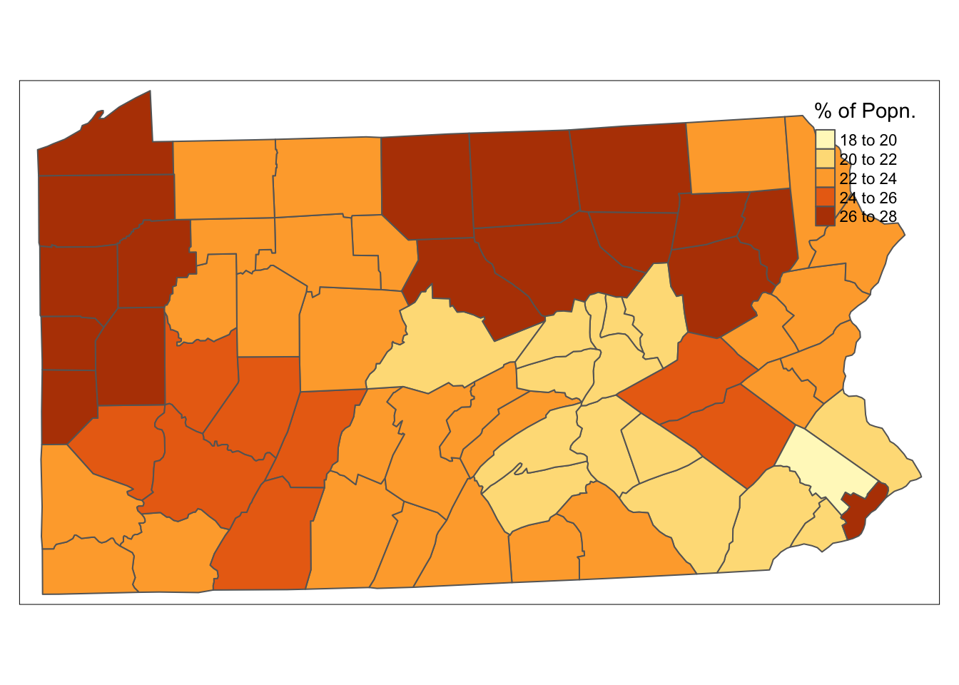
Using the packages tmap and tmaptools, for example, standard methods may be used to produce a choropleth map of smoking uptake in Pennsylvania. In the code below (all making use of techniques from earlier chapters), the map of Pennsylvania is transformed from geographical coordinates to UTM projection for zone 17. Note this has EPSG reference number 3724, as is used in the set_projection function. These are then used to create a chloropleth map as seen in figure . Note that this is produced on a notional window of 11 cm × 6 cm – you may have to resize the window or set par(mar=c(0,0,0,0)) to ensure the legend is visible.

# Make sure the necessary packages have been loaded
library(tmap)
library(tmaptools)
library(SpatialEpi)

# Read in the Pennsylvania lung cancer data
data(pennLC)
# Extract the SpatialPolygon info
penn.state.latlong <- pennLC$spatial.polygon

# Convert to UTM zone 17N
penn.state.utm <- set_projection(penn.state.latlong, 3724)
if ("sf" %in% class(penn.state.utm)) 
  penn.state.utm <- as(penn.state.utm,"Spatial")


# Obtain the smoking rates
penn.state.utm$smk <- pennLC$smoking$smoking * 100

# Draw a choropleth map of the smoking rates

tm_shape(penn.state.utm) + tm_polygons(col='smk',title='% of Popn.')

Figure 8.1: Smoking Uptake (Pennysylvania)

This produces a basic choropleth map of smoking rates in Pennsylvania. From this, it may be seen that these tend to show some degree of spatial clustering – counties having higher rates of uptake are generally near to other counties with higher rates of uptake, and similarly for lower rates of uptake. This is quite a common occurrence – and this kind of spatial clustering will be seen in the coming sections, for smoking rates, patterns in death rates, and in the classes used in the stratification of the population.