Chapter 9 R and Internet Data

require(devtools)

## Loading required package: devtools

install_version("eurostat", version = "3.1.5", repos = "http://cran.us.r-project.org")

## Downloading package from url: http://cran.us.r-project.org/src/contrib/Archive/eurostat/eurostat_3.1.5.tar.gz

library(eurostat)

9.1 Introduction

9.2 Direct Access to Data

fpe <- read.table("http://data.princeton.edu/wws509/datasets/effort.dat")
head(fpe)

##           setting effort change
## Bolivia        46      0      1
## Brazil         74      0     10
## Chile          89     16     29
## Colombia       77     16     25
## CostaRica      84     21     29
## Cuba           89     15     40

pairs(fpe,panel=panel.smooth)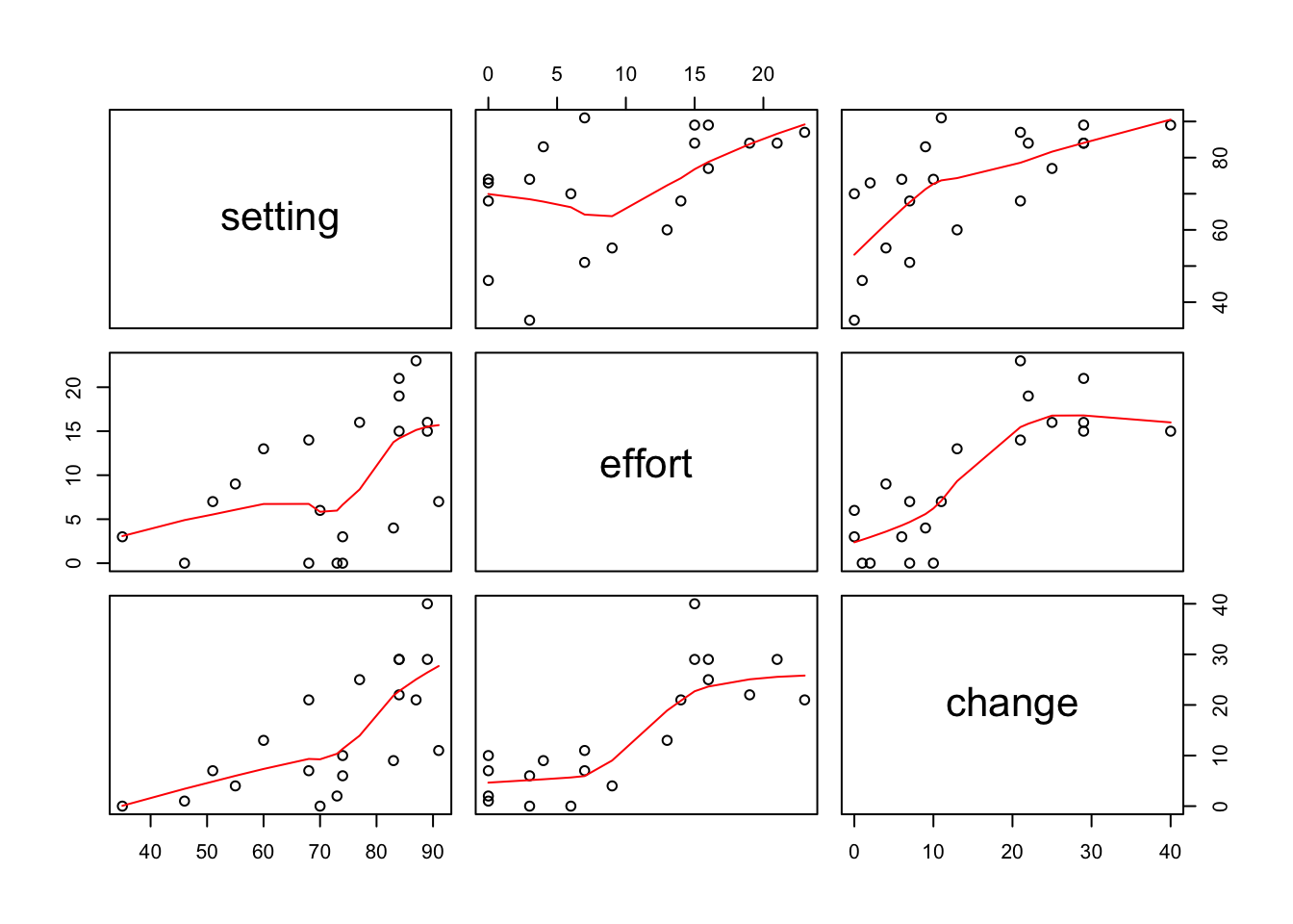

Figure 9.1: Scatterplot Matrix of Princeton Data

source("http://bioconductor.org/biocLite.R")
biocLite()

source("http://bioconductor.org/biocLite.R")
biocLite("Rgraphviz")

# The following two packages are required:
require(Rgraphviz)

## Loading required package: Rgraphviz

## Loading required package: graph

## Loading required package: BiocGenerics

## Loading required package: parallel

## 
## Attaching package: 'BiocGenerics'

## The following objects are masked from 'package:parallel':
## 
##     clusterApply, clusterApplyLB, clusterCall, clusterEvalQ,
##     clusterExport, clusterMap, parApply, parCapply, parLapply,
##     parLapplyLB, parRapply, parSapply, parSapplyLB

## The following objects are masked from 'package:stats':
## 
##     IQR, mad, sd, var, xtabs

## The following objects are masked from 'package:base':
## 
##     anyDuplicated, append, as.data.frame, basename, cbind,
##     colMeans, colnames, colSums, dirname, do.call, duplicated,
##     eval, evalq, Filter, Find, get, grep, grepl, intersect,
##     is.unsorted, lapply, lengths, Map, mapply, match, mget, order,
##     paste, pmax, pmax.int, pmin, pmin.int, Position, rank, rbind,
##     Reduce, rowMeans, rownames, rowSums, sapply, setdiff, sort,
##     table, tapply, union, unique, unsplit, which, which.max,
##     which.min

## Loading required package: grid

require(datasets)
# Load the state.x77 data
data(state)
# Which ones are 'connected' - ie abs correlation above 0.3
connected <- abs(cor(state.x77)) > 0.5 
# Create the graph - node names are the column names
conn <- graphNEL(colnames(state.x77))
# Populate with edges - join variables that are TRUE in 'connected'
for (i in colnames(connected)) {
  for (j in colnames(connected)) {
    if (i < j) {
      if (connected[i,j]) {
        conn <- addEdge(i,j,conn,1)}}}}
# Create a layout for the graph
conn <- layoutGraph(conn)
# Specify some drawing parameters
attrs <- list(node=list(shape="ellipse", 
                        fixedsize=FALSE, fontsize=12))
# Plot the graph
plot(conn,attrs=attrs)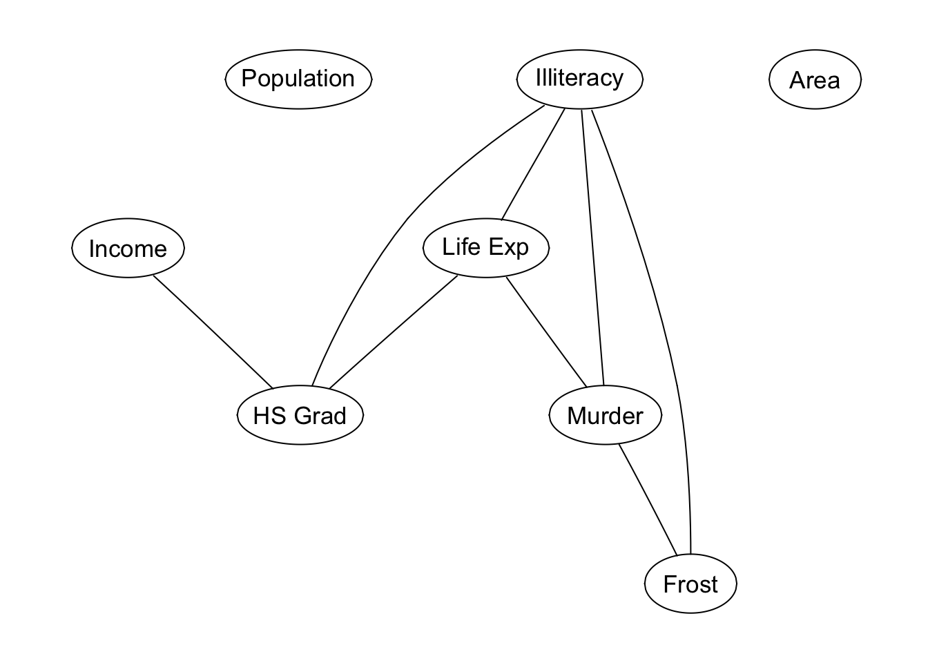

Figure 9.2: Illustration of Rgraphviz

9.3 Using `RCurl`

library(RCurl) # Load RCurl

## Loading required package: bitops

# Get the content of the URL and store it into 'temp'
stem <- 'https://www.gov.uk/government/uploads/system/uploads'
file1 <- '/attachment_data/file/15240/1871702.csv'
temp <- getURL(paste0(stem,file1))
# Use textConnection to read the content of temp
# as though it were a CSV file
imd <- read.csv(textConnection(temp))
# Check - this gives the first 10 column names of the data frame
head(colnames(imd),n=10)

## [1] "X.html..body.You.are.being..a.href.https...assets.publishing.service.gov.uk.government.uploads.system.uploads.attachment_data.file.15240.1871702.csv.redirected..a....body...html."

read.csv.https <- function(url) {
  temp <- getURL(url)
  return(read.csv(textConnection(temp)))
}

# Download the csv dataand put it into 'imd2'
imd <- read.csv(paste0(stem,file1))
# Modify the margins around the plot, to fit the GOR
# names into the left-hand margin
par(mar=c(5,12,4,2) + 0.1)
# Create the boxplot. The 'las' parameter specificies y-axis 
# labelling is horizontal, x-axis is vertical
boxplot(IMD.SCORE~GOR.NAME,data=imd,horizontal=TRUE,las=2)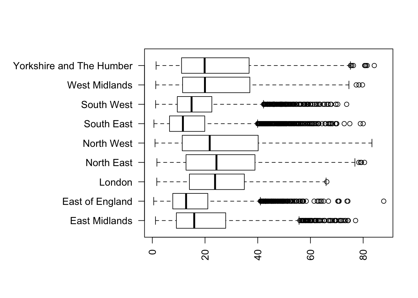

Figure 9.3: Boxplot of IMDs by Goverment Office Regions

9.4 Working with APIs

crimes.buf <- getForm(
  "http://data.police.uk/api/crimes-street/all-crime",
  lat=53.401422,
  lng=-2.965075,
  date="2016-04")

require(rjson)

## Loading required package: rjson

crimes <- fromJSON(crimes.buf)

crimes[[1]]

## $category
## [1] "anti-social-behaviour"
## 
## $location_type
## [1] "Force"
## 
## $location
## $location$latitude
## [1] "53.403924"
## 
## $location$street
## $location$street$id
## [1] 910391
## 
## $location$street$name
## [1] "On or near Back Bold Street"
## 
## 
## $location$longitude
## [1] "-2.979198"
## 
## 
## $context
## [1] ""
## 
## $outcome_status
## NULL
## 
## $persistent_id
## [1] "f928374af70088b30cbc70ff0f44c0caf40bb2040e22783cfb88b5bcd9d4bda7"
## 
## $id
## [1] 48502675
## 
## $location_subtype
## [1] ""
## 
## $month
## [1] "2016-04"

getLonLat <- function(x) as.numeric(c(x$location$longitude,
                                      x$location$latitude))
crimes.loc <- t(sapply(crimes,getLonLat))
head(crimes.loc)

##           [,1]     [,2]
## [1,] -2.979198 53.40392
## [2,] -2.987014 53.40565
## [3,] -2.981499 53.40391
## [4,] -2.988220 53.40187
## [5,] -2.983495 53.40569
## [6,] -2.949829 53.39618

getAttr <- function(x) c(
  x$category,
  x$location$street$name,
  x$location_type)
crimes.attr <- as.data.frame(t(sapply(crimes,getAttr)))
colnames(crimes.attr) <- c("category","street","location_type")
head(crimes.attr)

##                category                      street location_type
## 1 anti-social-behaviour On or near Back Bold Street         Force
## 2 anti-social-behaviour    On or near Shopping Area         Force
## 3 anti-social-behaviour        On or near Roe Alley         Force
## 4 anti-social-behaviour    On or near Canning Place         Force
## 5 anti-social-behaviour    On or near Shopping Area         Force
## 6 anti-social-behaviour  On or near Maitland Street         Force

library(sp)
crimes.pts <- SpatialPointsDataFrame(crimes.loc,crimes.attr)
# Specify the projection - in this case just geographical coordinates
proj4string(crimes.pts) <- CRS("+proj=longlat")
# Note that 'head' doesn't work on SpatialPointsDataFrames
crimes.pts[1:6,]

##             coordinates              category                      street
## 1 (-2.979198, 53.40392) anti-social-behaviour On or near Back Bold Street
## 2 (-2.987014, 53.40565) anti-social-behaviour    On or near Shopping Area
## 3 (-2.981499, 53.40391) anti-social-behaviour        On or near Roe Alley
## 4  (-2.98822, 53.40187) anti-social-behaviour    On or near Canning Place
## 5 (-2.983495, 53.40569) anti-social-behaviour    On or near Shopping Area
## 6 (-2.949829, 53.39618) anti-social-behaviour  On or near Maitland Street
##   location_type
## 1         Force
## 2         Force
## 3         Force
## 4         Force
## 5         Force
## 6         Force

asb.pts <- crimes.pts[crimes.pts$category=="anti-social-behaviour",]

cda.pts <- crimes.pts[crimes.pts$category=="criminal-damage-arson",]

require(tmap)

## Loading required package: tmap

require(tmaptools)

## Loading required package: tmaptools

asb_cda.pts <- rbind(asb.pts,cda.pts)
asb_cda.pts$category <- as.character(asb_cda.pts$category)
tm_shape(asb_cda.pts) + tm_dots(col='category',title='Crime Type',
                                labels=c("Antisocial Behaviour","Criminal Damage"),
                                palette=c('indianred','dodgerblue'),size=0.1)

## Linking to GEOS 3.6.1, GDAL 2.1.3, PROJ 4.9.3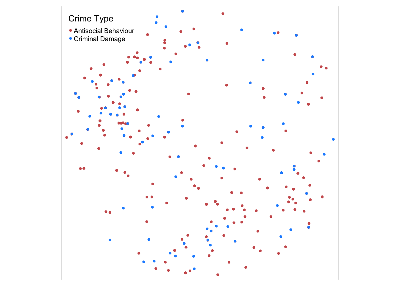

Figure 9.4: Locations of anti-social behaviour and criminal damage/arson incidents

tmap_mode('view')

## tmap mode set to interactive viewing

tm_shape(asb_cda.pts) + tm_dots(col='category',title='Crime Type',
                                labels=c("Antisocial Behaviour","Criminal Damage"),
                                palette=c('indianred','dodgerblue'),size=0.02)

9.5 Creating a Statistical ‘Mashup’

terr3bed.buf <- getForm("https://api.nestoria.co.uk/api",
  action='search_listings',
  place_name='liverpool',
  encoding='json',
  listing_type='buy',
  number_of_results=50,
  bedroom_min=3,bedroom_max=3,
  keywords='terrace')

## Warning in testCurlOptionsInFormParameters(.params): Found possible curl
## options in form parameters: encoding

terr3bed <- fromJSON(terr3bed.buf)

getHouseAttr <- function(x) {
  as.numeric(c(x$price/1000,x$longitude,x$latitude))
}

terr3bed.attr <- as.data.frame(t(sapply(terr3bed$response$listings,
                                        getHouseAttr)))

colnames(terr3bed.attr) <- c("price","longitude","latitude")
head(terr3bed.attr)

##    price longitude latitude
## 1 120.00 -2.940470 53.41720
## 2  95.00 -2.924914 53.40125
## 3 160.00 -2.859435 53.38674
## 4 195.00 -2.922263 53.38855
## 5  89.95 -2.922261 53.41416
## 6  85.00 -2.932500 53.43038

# Create an extra column to contain burglary rates
terr3bed.attr <- transform(terr3bed.attr,burgs=0)

# For each house in the data frame
for (i in 1:50) {
  # Firstly obtain crimes in a 1-mile radius of the houses
  # latitude and longitude and decode it from JSON form
  crimes.near <- getForm(
  "http://data.police.uk/api/crimes-street/all-crime",
  lat=terr3bed.attr$latitude[i],
  lng=terr3bed.attr$longitude[i],
  date="2016-04")
  crimes.near <- fromJSON(crimes.near)
  crimes.near <- as.data.frame(t(sapply(crimes.near,getAttr)))
  # Then from the 'category' column count the number of burlaries
  # and assign it to the burgs column
  terr3bed.attr$burgs[i] <- sum(crimes.near[,1] == 'burglary')
  # Pause before running next API request - to avoid overloading
  # the server
  Sys.sleep(0.7)
  # Note this stage may cause the code to take a minute or two to run
}

library(ggplot2)
ggplot(terr3bed.attr,aes(x=burgs,y=price)) + geom_point() +
  geom_smooth(span=1) + 
  labs(x='Burglaries in a 1-Mile Radius',
       y='House Price (1000s Pounds)')

## `geom_smooth()` using method = 'loess' and formula 'y ~ x'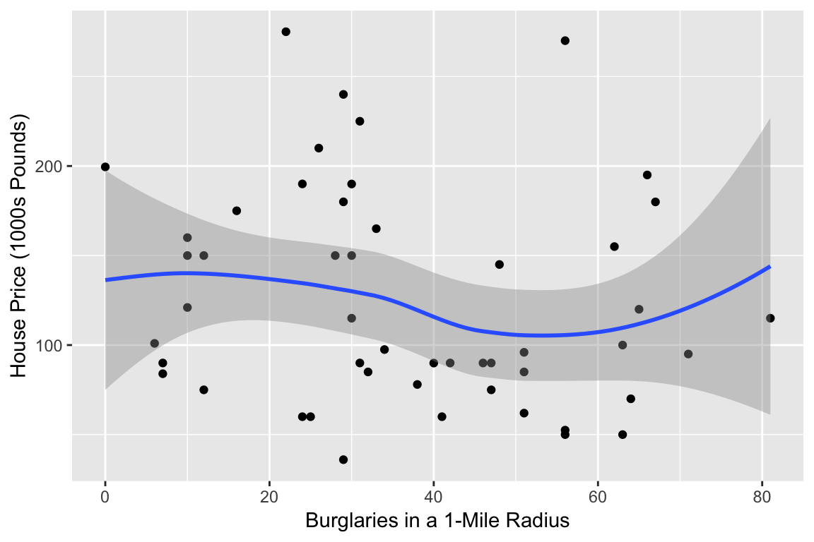

Figure 9.5: Scatter plot of Burglary Rate vs. House Price

9.6 Using Specific Packages

library(eurostat)
tgs00026 <- get_eurostat("tgs00026", time_format = "raw")

## Table tgs00026 cached at /var/folders/t4/3d2rv9_10wx7_xckhgslrmv00000gn/T//RtmpNT6Mtr/eurostat/tgs00026_raw_code_TF.rds

head(tgs00026)

## # A tibble: 6 x 5
##   unit     na_item geo   time  values
##   <fct>    <fct>   <fct> <chr>  <dbl>
## 1 PPCS_HAB B6N     AT11  2005   18100
## 2 PPCS_HAB B6N     AT12  2005   18900
## 3 PPCS_HAB B6N     AT13  2005   19400
## 4 PPCS_HAB B6N     AT21  2005   17800
## 5 PPCS_HAB B6N     AT22  2005   17800
## 6 PPCS_HAB B6N     AT31  2005   18400

tgs00026_05 <- tgs00026[tgs00026$time=='2005',]
tgs00026_10 <- tgs00026[tgs00026$time=='2010',]
tgs00026_10$delta <- 
  100*(tgs00026_10$values - tgs00026_05$values)/tgs00026_05$values

tgs00026_10$country <- substr(as.character(tgs00026_10$geo),1,2)

ggplot(tgs00026_10,aes(x=country,y=delta)) + geom_boxplot() +
  labs(x="Country",y="% Change in Household\n Income 2005-2010")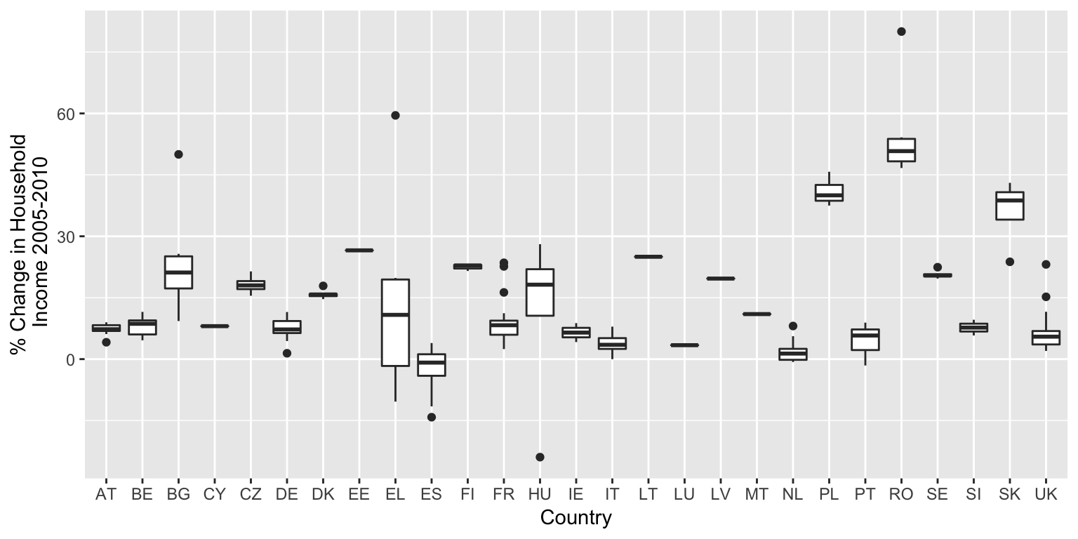

Figure 9.6: Box plots of disposable income change 2005-10 by country (Eurostat data).

library(forcats)
tgs00026_10$country <- 
  fct_reorder(tgs00026_10$country,tgs00026_10$delta,median)
ggplot(tgs00026_10,aes(x=country,y=delta)) + geom_boxplot() + 
  labs(x="Country",y="% Change in Household\n Income 2005-2010")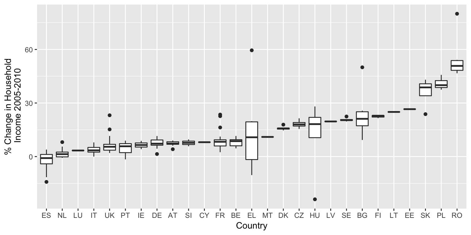

Figure 9.7: Median ordered box plots of disposable income change 2005-10 by country.

tmap_mode('plot')

## tmap mode set to plotting

tgs_es <- tgs00026_10[tgs00026_10$country=='ES',]
tgs_map <- merge_eurostat_geodata(data = tgs_es, geocolumn = "geo",
              resolution = "1", output_class = "spdf", all_regions = FALSE)

## 
##       COPYRIGHT NOTICE
## 
##       When data downloaded from this page 
##       <http://ec.europa.eu/eurostat/web/gisco/geodata/reference-data/administrative-units-statistical-units>
##       is used in any printed or electronic publication, 
##       in addition to any other provisions 
##       applicable to the whole Eurostat website, 
##       data source will have to be acknowledged 
##       in the legend of the map and 
##       in the introductory page of the publication 
##       with the following copyright notice:
## 
##       - EN: (C) EuroGeographics for the administrative boundaries
##       - FR: (C) EuroGeographics pour les limites administratives
##       - DE: (C) EuroGeographics bezuglich der Verwaltungsgrenzen
## 
##       For publications in languages other than 
##       English, French or German, 
##       the translation of the copyright notice 
##       in the language of the publication shall be used.
## 
##       If you intend to use the data commercially, 
##       please contact EuroGeographics for 
##       information regarding their licence agreements.
##

## SpatialPolygonDataFrame at resolution 1: 01  cached at:  /var/folders/t4/3d2rv9_10wx7_xckhgslrmv00000gn/T//RtmpqSz3Qb/eurostat/spdf01.RData

tm_shape(tgs_map) + tm_polygons(col='delta',title="Change (%)") +
  tm_style("col_blind") + tm_credits("(C) EuroGeographics for the administrative boundaries") + tm_layout(legend.position = c("left", "top"))

## Variable "delta" contains positive and negative values, so midpoint is set to 0. Set midpoint = NA to show the full spectrum of the color palette.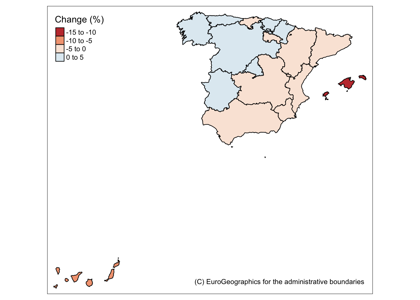

$Household Income Change (\%, 2005-10) In Spain$

Figure 9.8: Household Income Change (%, 2005-10) In Spain

tmap_mode('plot')

## tmap mode set to plotting

tgs_mlmap <- tgs_map[!(tgs_map$NUTS_ID %in% c("ES70","ES53")),]
tm_shape(tgs_mlmap) + tm_polygons(col='delta',title="Change (%)") +
  tm_style_col_blind() + 
  tm_layout(legend.position=c("right","bottom")) +
  tm_credits("(C) EuroGeographics for the administrative boundaries")

## Warning in tm_style_col_blind(): tm_style_col_blind is deprecated as of
## tmap version 2.0. Please use tm_style("col_blind", ...) instead

## Variable "delta" contains positive and negative values, so midpoint is set to 0. Set midpoint = NA to show the full spectrum of the color palette.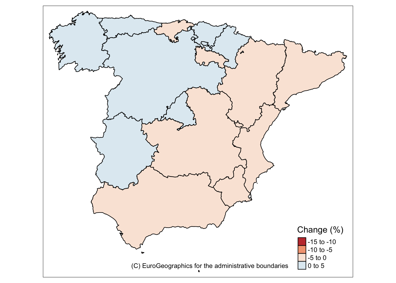

$Household Income Change (\%, 2005-10) In Mainland Spain$

Figure 9.9: Household Income Change (%, 2005-10) In Mainland Spain

9.7 Web Scraping

grepl('Chris[0-9]*',c('Chris','Lex','Chris1999','Chris Brunsdon'))

## [1]  TRUE FALSE  TRUE  TRUE

grep('Chris[0-9]*',c('Chris','Lex','Chris1999','Chris Brunsdon'))

## [1] 1 3 4

grep('Chris[0-9]*',c('Chris','Lex','Chris1999','Chris Brunsdon'),
     value=TRUE)

## [1] "Chris"          "Chris1999"      "Chris Brunsdon"

9.7.1 Scraping Train Times

web.buf <- readLines(
  "https://traintimes.org.uk/durham/leicester/00:00/monday")

times <- grep("strong.*[0-2][0-9]:[0-5][0-9].*[0-2][0-9]:[0-5][0-9]",
              web.buf,value=TRUE)

locs <- gregexpr("[0-2][0-9]:[0-5][0-9]",times)
# Show the match information for times[1]
locs[[1]]

## [1] 46 60
## attr(,"match.length")
## [1] 5 5
## attr(,"index.type")
## [1] "chars"
## attr(,"useBytes")
## [1] TRUE

timedata <- matrix(0,length(locs),4)
ptr <- 1
for (loc in locs) {
  timedata[ptr,1] <- as.numeric(substr(times[ptr],loc[1],loc[1]+1))
  timedata[ptr,2] <- as.numeric(substr(times[ptr],loc[1]+3,loc[1]+4))
  timedata[ptr,3] <- as.numeric(substr(times[ptr],loc[2],loc[2]+1))
  timedata[ptr,4] <- as.numeric(substr(times[ptr],loc[2]+3,loc[2]+4))
  ptr <- ptr + 1
}
colnames(timedata) <- c('h1','m1','h2','m2')
timedata <- transform(timedata,duration = h2 + m2/60 - h1 - m1/60 )
timedata

##   h1 m1 h2 m2 duration
## 1  4 59  8 24 3.416667
## 2  4 59  8 31 3.533333
## 3  6 38  9 18 2.666667
## 4  6 44  9 46 3.033333
## 5  6 57 10  0 3.050000