Chapter 8 Localised Spatial Analysis

8.1 Introduction

8.2 Setting Up The Data Used in This Chapter

# Load tmap, tmaptools packages
require(tmap)
require(tmaptools)

# read in the shapefile for North Carolina SIDS (its in epsg:4326)
nc.sids <- read_shape(system.file("shapes/sids.shp",
                                  package="spData")[1],
                      current.projection=4326)

# Transform to EPSG 2264 - and units in miles. We need the full proj4 string here to specify units
nc.sids.p <- set_projection(nc.sids,"+init=epsg:2264 +units=mi")

# Plot North Carolina
tm_shape(nc.sids.p,unit='miles') + tm_borders() + tm_scale_bar(position = c("left","bottom"))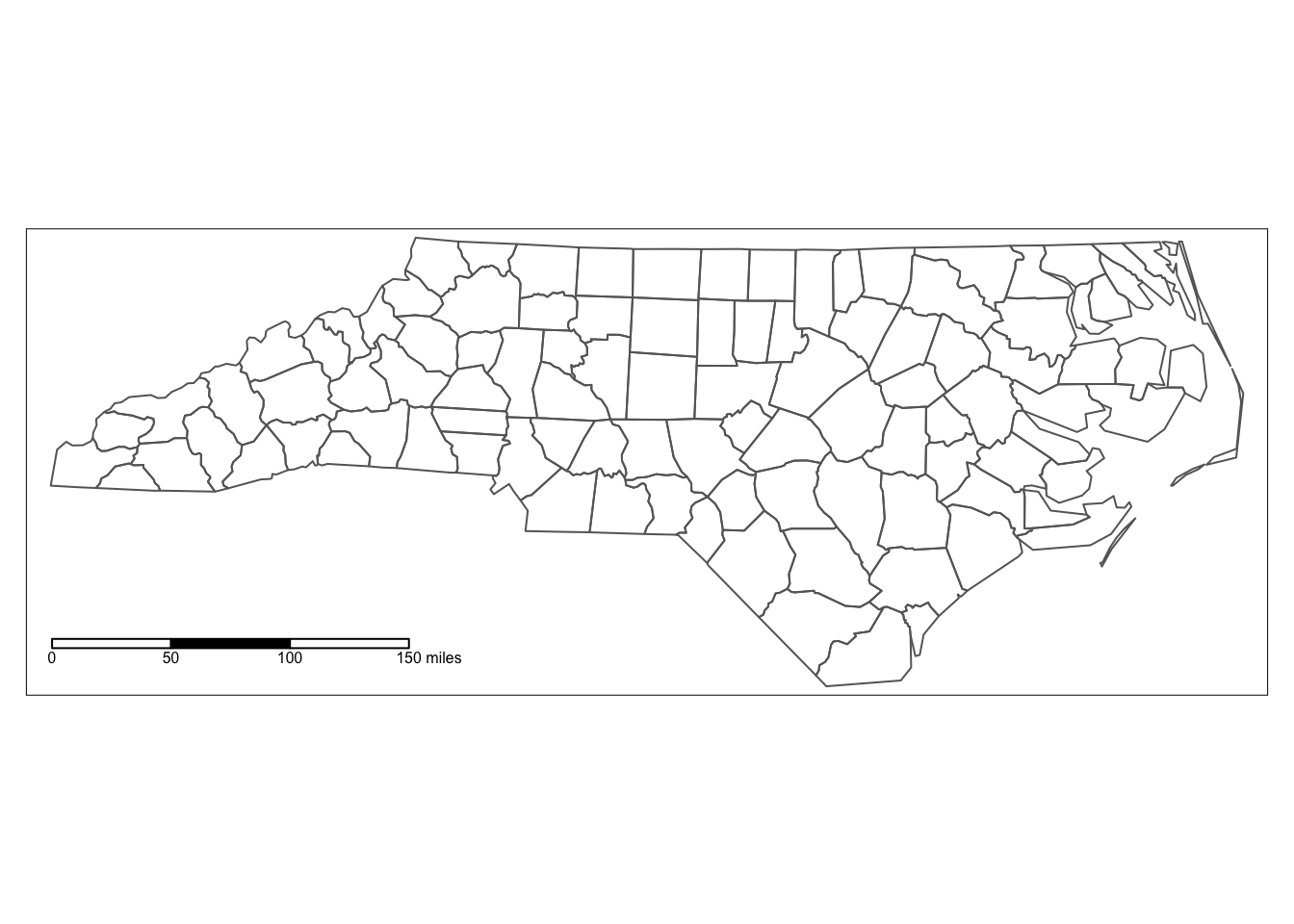

Figure 8.1: North Carolina SIDS Data, County Map

8.2.1 Local Indicators of Spatial Association

require(spdep)
# Compute the listw object for the North Carolina polygons
# Make sure nc.sids.p is in SpatialPolygonsDataFrame format
if ("sf" %in% class(nc.sids.p)) nc.sids.p <- as(nc.sids.p,"Spatial")
nc.lw <- nb2listw(poly2nb(nc.sids.p))
# Compute the SIDS rates (per 1000 births) for 1979
nc.sids.p$sidspm79 <- 1000*nc.sids.p$SID79/nc.sids.p$BIR79
# Compute the local Moran's I
nc.sids.p$lI <- localmoran(nc.sids.p$sidspm79,nc.lw)[,1]
tm_shape(nc.sids.p,unit='miles') + 
  tm_polygons(col='lI',title="Local Morans I",legend.format=list(flag="+")) +
  tm_style_col_blind() + tm_scale_bar(width=0.15) +
  tm_layout(legend.position = c("left","bottom"),
            legend.text.size=0.4)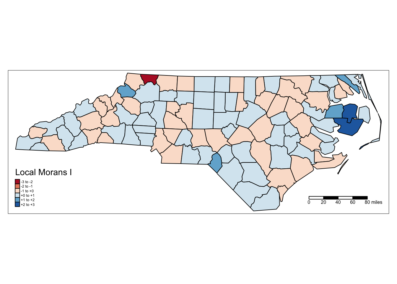

Figure 8.2: Standardised local Moran’s-\(I\)

# Create the local p-values
nc.sids.p$pval <- localmoran(nc.sids.p$sidspm79,nc.lw)[,5]
# Draw the map
tm_shape(nc.sids.p,unit='miles') + 
 tm_polygons(col='pval',title="p-value",breaks=c(0,0.01,0.05,0.10,1),
             border.col = "black",
             palette = "-Greens") +
 tm_scale_bar(width=0.15) + 
 tm_layout(legend.position = c("left","bottom"))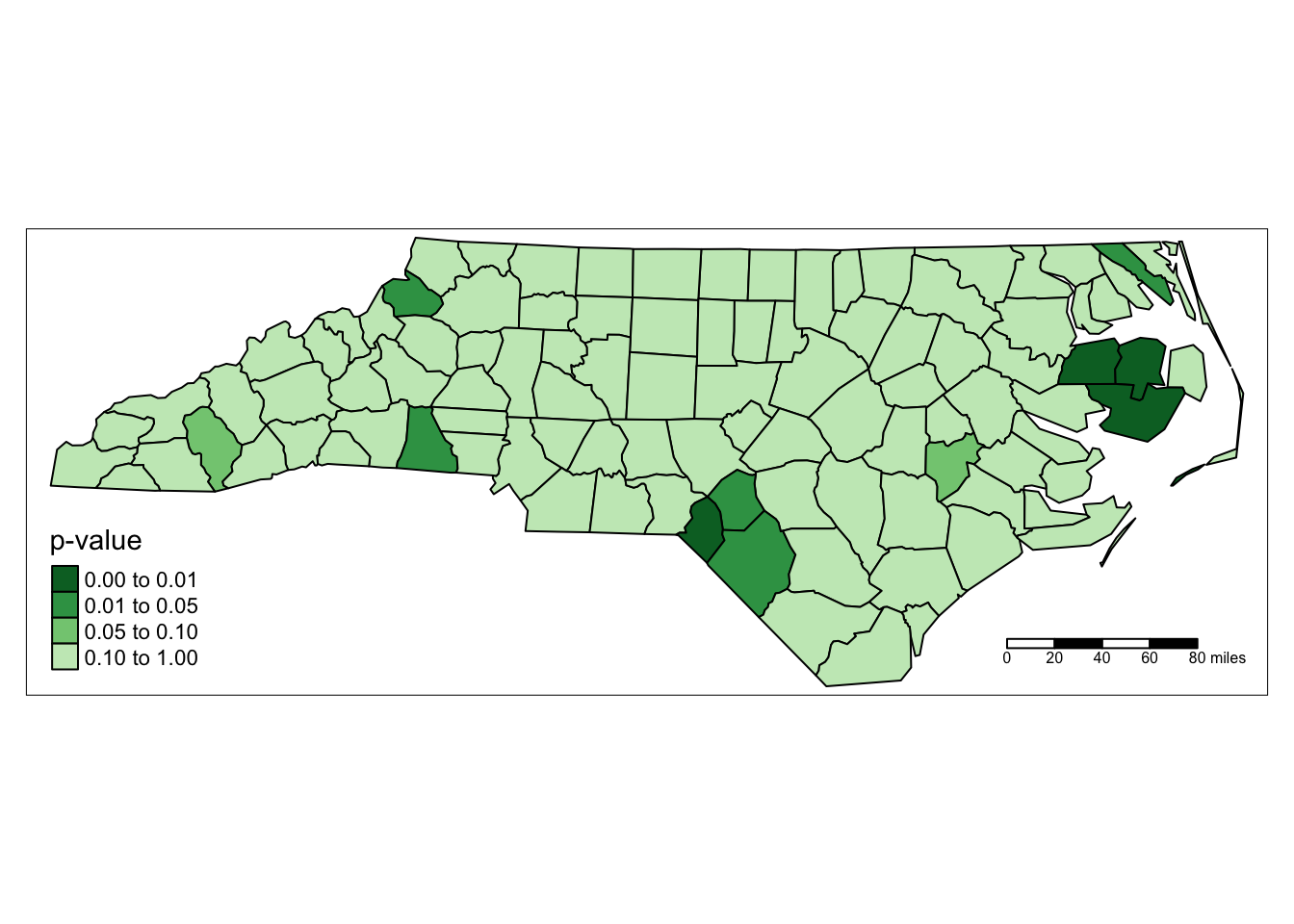

Figure 8.3: Local Moran’s-\(I\) \(p\)-values

Self Test Question 1 Verify the significance figures above by selecting and listing the counties for which \(p<0.05\).

8.3 Further Issues With The Above Analysis

8.3.1 Multiple Hypothesis Testing

# Create the adjusted p-value
nc.sids.p$pval_bonf <- p.adjust(nc.sids.p$pval,method='bonferroni')
# Draw the map
tm_shape(nc.sids.p,unit='miles') + 
 tm_polygons(col='pval_bonf',title="p-value",breaks=c(0,0.01,0.05,0.10,1),
             border.col = "black",
             palette = "-BuGn") +
 tm_scale_bar(width=0.15) + 
 tm_layout(legend.position = c("left","bottom"))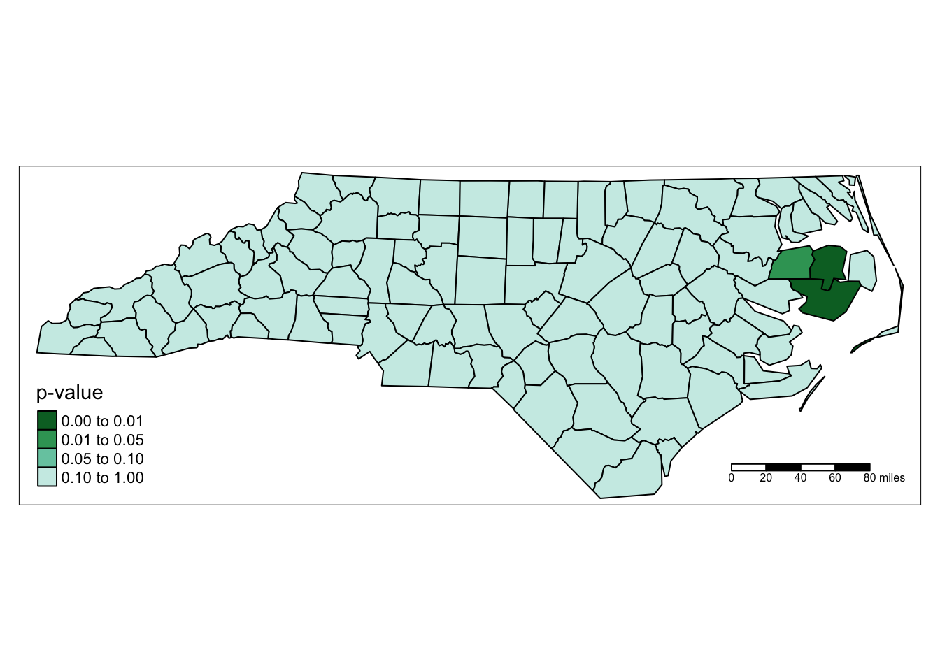

Figure 8.4: Local Moran’s-\(I\) Bonferroni adjusted \(p\)-values