Chapter 2 Data and Plots
2.2 The basic ingredients of R: variables and assignment
# examples of simple assignment
x <- 5
y <- 4
# the variables can be used in other operations
x+y
[1] 9# including defining new variables
z <- x + y
z[1] 9# which can then be passed to other functions
sqrt(z)[1] 3# example of Vector assignment
tree.heights <- c(4.3,7.1,6.3,5.2,3.2,2.1)
tree.heights[1] 4.3 7.1 6.3 5.2 3.2 2.1tree.heights**2[1] 18.49 50.41 39.69 27.04 10.24 4.41sum(tree.heights)[1] 28.2mean(tree.heights)[1] 4.7max.height <- max(tree.heights)
max.height[1] 7.1tree.heights[1] 4.3 7.1 6.3 5.2 3.2 2.1tree.heights [1] # first element[1] 4.3tree.heights[1:3] # a subset of elements 1 to 3[1] 4.3 7.1 6.3sqrt(tree.heights[1:3]) #square roots of the subset[1] 2.073644 2.664583 2.509980tree.heights[c(5,3,2)] # a subset of elements 5,3,2: note the ordering[1] 3.2 6.3 7.1# examples of Character Variable assignment
name <- "Lex Comber"
name[1] "Lex Comber"# these can be assigned to a vector of character variables
cities <- c("Leicester","Newcastle","London","Leeds","Exeter")
cities[1] "Leicester" "Newcastle" "London" "Leeds"
[5] "Exeter" length(cities)[1] 5# an example of a Logical Variable
northern <- c(FALSE, TRUE, FALSE, TRUE, FALSE)
northern[1] FALSE TRUE FALSE TRUE FALSE# this can be used to subset other variables
cities[northern][1] "Newcastle" "Leeds" 2.3 Data types and Data classes
2.3.1 Data Types in R
2.3.1.1 Characters
character(8) [1] "" "" "" "" "" "" "" ""# conversion
as.character("8") [1] "8"# tests
is.character(8)[1] FALSEis.character("8")[1] TRUE2.3.1.2 Numeric
numeric(8)[1] 0 0 0 0 0 0 0 0# conversions
as.numeric(c("1980","-8","Geography"))[1] 1980 -8 NAas.numeric(c(FALSE,TRUE))[1] 0 1# tests
is.numeric(c(8, 8))[1] TRUEis.numeric(c(8, 8, 8, "8"))[1] FALSE2.3.1.3 Logical
logical(7)[1] FALSE FALSE FALSE FALSE FALSE FALSE FALSE# conversion
as.logical(c(7, 5, 0, -4,5))[1] TRUE TRUE FALSE TRUE TRUE# TRUE and FALSE can be converted to 1 and 0
as.logical(c(7,5,0,-4,5)) * 1[1] 1 1 0 1 1as.logical(c(7,5,0,-4,5)) + 0[1] 1 1 0 1 1# different ways to declare TRUE and FALSE
as.logical(c("True","T","FALSE","Raspberry","9","0", 0))[1] TRUE TRUE FALSE NA NA NA NAdata <- c(3, 6, 9, 99, 54, 32, -102)
# a logical test
index <- (data > 10)
index[1] FALSE FALSE FALSE TRUE TRUE TRUE FALSE# used to subset data
data[index][1] 99 54 32sum(data)[1] 101sum(data[index])[1] 1852.3.2 Data Classes in R
2.3.2.1 Vectors
# defining vectors
vector(mode = "numeric", length = 8)
[1] 0 0 0 0 0 0 0 0vector(length = 8)[1] FALSE FALSE FALSE FALSE FALSE FALSE FALSE FALSE# testing and conversion
tmp <- data.frame(a=10:15, b=15:20)
is.vector(tmp)[1] FALSEas.vector(tmp)$a
[1] 10 11 12 13 14 15
$b
[1] 15 16 17 18 19 202.3.2.2 Matrices
# defining matrices
matrix(ncol = 2, nrow = 0)
[,1] [,2]matrix(1:6) [,1]
[1,] 1
[2,] 2
[3,] 3
[4,] 4
[5,] 5
[6,] 6matrix(1:6, ncol = 2) [,1] [,2]
[1,] 1 4
[2,] 2 5
[3,] 3 6# conversion and test
as.matrix(6:3) [,1]
[1,] 6
[2,] 5
[3,] 4
[4,] 3is.matrix(as.matrix(6:3))[1] TRUEflow <- matrix(c(2000, 1243, 543, 1243, 212, 545,
654, 168, 109), c(3,3), byrow=TRUE)
# Rows and columns can have names, not just 1,2,3,...
colnames(flow) <- c("Leeds", "Maynooth"," Elsewhere")
rownames(flow) <- c("Leeds", "Maynooth", "Elsewhere")
# examine the matrix
flow Leeds Maynooth Elsewhere
Leeds 2000 1243 543
Maynooth 1243 212 545
Elsewhere 654 168 109# and functions exist to summarise
outflows <- rowSums(flow)
outflows Leeds Maynooth Elsewhere
3786 2000 931 z <- c(6,7,8)
names(z) <- c("Newcastle","London","Manchester")
z Newcastle London Manchester
6 7 8 ?sum
help(sum)
# Create a variable to pass to other summary functions
x <- matrix(c(3,6,8,8,6,1,-1,6,7),c(3,3),byrow=TRUE)
# Sum over rows
rowSums(x)
# Sum over columns
colSums(x)
# Calculate column means
colMeans(x)
# Apply function over rows (1) or columns (2) of x
apply(x,1,max)
# Logical operations to select matrix elements
x[,c(TRUE,FALSE,TRUE)]
# Add up all of the elements in x
sum(x)
# Pick out the leading diagonal
diag(x)
# Matrix inverse
solve(x)
# Tool to handle rounding
zapsmall(x %*% solve(x)) 2.3.2.3 Factors
# a vector assignment
house.type <- c("Bungalow", "Flat", "Flat",
    "Detached", "Flat", "Terrace", "Terrace")
# a factor assignment
house.type <- factor(c("Bungalow", "Flat",
    "Flat", "Detached", "Flat", "Terrace", "Terrace"),
    levels=c("Bungalow","Flat","Detached","Semi","Terrace"))
house.type
[1] Bungalow Flat Flat Detached Flat Terrace
[7] Terrace
Levels: Bungalow Flat Detached Semi Terrace# table can be used to summarise
table(house.type)house.type
Bungalow Flat Detached Semi Terrace
1 3 1 0 2 # 'levels' control what can be assigned
house.type <- factor(c("People Carrier", "Flat",
"Flat", "Hatchback", "Flat", "Terrace", "Terrace"),
levels=c("Bungalow","Flat","Detached","Semi","Terrace"))
house.type[1] <NA> Flat Flat <NA> Flat Terrace Terrace
Levels: Bungalow Flat Detached Semi Terrace2.3.2.4 Ordering
income <-factor(c("High", "High", "Low", "Low",
    "Low", "Medium", "Low", "Medium"),
    levels=c("Low", "Medium", "High"))
income > "Low"
[1] NA NA NA NA NA NA NA NA# 'levels' in 'ordered' defines a relative order
income <-ordered(c("High", "High", "Low", "Low",
"Low", "Medium", "Low", "Medium"),
levels=c("Low", "Medium", "High"))
income > "Low"[1] TRUE TRUE FALSE FALSE FALSE TRUE FALSE TRUEsort(income)2.3.2.5 Lists
tmp.list <- list("Lex Comber",c(2015, 2018),
    "Lecturer", matrix(c(6,3,1,2), c(2,2)))
tmp.list
[[1]]
[1] "Lex Comber"
[[2]]
[1] 2015 2018
[[3]]
[1] "Lecturer"
[[4]]
     [,1] [,2]
[1,]    6    1
[2,] 3 2# elements of the list can be selected
tmp.list[[4]] [,1] [,2]
[1,] 6 1
[2,] 3 2employee <- list(name="Lex Comber", start.year = 2015,
position="Professor")
employee$name
[1] "Lex Comber"
$start.year
[1] 2015
$position
[1] "Professor"append(tmp.list, list(c(7,6,9,1)))# lappy with different functions
lapply(tmp.list[[2]], is.numeric)
lapply(tmp.list, length)2.3.2.6 Defining your own Classes
employee <- list(name="Lex Comber", start.year = 2015,
position="Professor")class(employee) <- "staff"print.staff <- function(x) {
cat("Name: ",x$name,"\n")
cat("Start Year: ",x$start.year,"\n")
cat("Job Title: ",x$position,"\n")}
# an example of the print class
print(employee)Name: Lex Comber
Start Year: 2015
Job Title: Professor print(unclass(employee))$name
[1] "Lex Comber"
$start.year
[1] 2015
$position
[1] "Professor"2.3.2.7 Classes in Lists
new.staff <- function(name,year,post) {
  result <- list(name=name, start.year=year, position=post)
  class(result) <- "staff"
  return(result)}
leeds.uni <- vector(mode='list',3)
# assign values to elements in the list
leeds.uni[[1]] <- new.staff("Heppenstall, Alison", 2017,"Professor")
leeds.uni[[2]] <- new.staff("Comber, Lex", 2015,"Professor")
leeds.uni[[3]] <- new.staff("Langlands, Alan", 2014,"VC")And the list can be examined by entering:
leeds.uni2.3.2.8 data.frame vs tibble
df <- data.frame(dist = seq(0,400, 100),
  city = c("Leeds", "Nottingham", "Leicester", "Durham", "Newcastle"))
str(df)
'data.frame': 5 obs. of 2 variables:
$ dist: num 0 100 200 300 400
$ city: chr "Leeds" "Nottingham" "Leicester" "Durham" ...df$citydf <- data.frame(dist = seq(0,400, 100),
city = c("Leeds", "Nottingham", "Leicester", "Durham", "Newcastle"),
stringsAsFactors = FALSE)
str(df)'data.frame': 5 obs. of 2 variables:
$ dist: num 0 100 200 300 400
$ city: chr "Leeds" "Nottingham" "Leicester" "Durham" ...tb <- tibble(dist = seq(0,400, 100),
city = c("Leeds", "Nottingham", "Leicester", "Durham", "Newcastle"))df$ci[1] "Leeds" "Nottingham" "Leicester" "Durham"
[5] "Newcastle" tb$ciNULL# 1 column
df[,2]
tb[,2]
class(df[,2])
class(tb[,2])
# 2 columns
df[,1:2]
tb[,1:2]
class(df[,1:2])
class(tb[,1:2])data.frame(tb)
as_tibble(df) cbind(df, Pop = c(700,250,230,150,1200)) dist city Pop
1 0 Leeds 700
2 100 Nottingham 250
3 200 Leicester 230
4 300 Durham 150
5 400 Newcastle 1200cbind(tb, Pop = c(700,250,230,150,1200)) dist city Pop
1 0 Leeds 700
2 100 Nottingham 250
3 200 Leicester 230
4 300 Durham 150
5 400 Newcastle 1200vignette("tibble")2.3.3 Self-Test Questions
2.3.3.1 Factors
colours <- factor(c("red","blue","red","white",
    "silver","red","white","silver",
    "red","red","white","silver","silver"),
    levels=c("red","blue","white","silver","black"))
Self-Test Question 1:
colours[4] <- "orange"
colours
colours <- factor(c("red","blue","red","white",
"silver","red","white","silver",
"red","red","white","silver","silver"),
levels=c("red","blue","white","silver","black"))
table(colours)colours
red blue white silver black
5 1 3 4 0 colours2 <-c("red","blue","red","white",
"silver","red","white","silver",
"red","red","white","silver")
# Now, make the table
table(colours2)colours2
blue red silver white
1 5 3 3 Self-Test Question 2
car.type <- factor(c("saloon","saloon","hatchback",
    "saloon","convertible","hatchback","convertible",
    "saloon", "hatchback","saloon", "saloon",
    "saloon","hatchback"),
levels=c("saloon","hatchback","convertible"))table(car.type, colours) colours
car.type red blue white silver black
saloon 2 1 2 2 0
hatchback 3 0 0 1 0
convertible 0 0 1 1 0crosstab <- table(car.type,colours)Self-Test Question 3
engine <- ordered(c("1.1litre","1.3litre","1.1litre",
    "1.3litre","1.6litre","1.3litre","1.6litre",
    "1.1litre","1.3litre","1.1litre", "1.1litre",
    "1.3litre","1.3litre"),
    levels=c("1.1litre","1.3litre","1.6litre"))
engine > "1.1litre" [1] FALSE TRUE FALSE TRUE TRUE TRUE TRUE FALSE TRUE
[10] FALSE FALSE TRUE TRUESelf-Test Question 4
2.3.3.2 Matrices
dim(crosstab) # Matrix dimensions[1] 3 5rowSums(crosstab) # Row sums saloon hatchback convertible
7 4 2 colnames(crosstab) # Column names[1] "red" "blue" "white" "silver" "black" apply(crosstab,1,max) saloon hatchback convertible
2 3 1 apply(crosstab,2,max) red blue white silver black
3 1 2 2 0 example <- c(1.4,2.6,1.1,1.5,1.2)
which.max(example)[1] 2Self-Test Question 5
Self-Test Question 6
levels(engine)[1] "1.1litre" "1.3litre" "1.6litre"levels(colours)[which.max(crosstab[,1])][1] "blue"colnames(crosstab)[which.max(crosstab[,1])][1] "blue"colnames(crosstab)[1] "red" "blue" "white" "silver" "black" crosstab[,1] saloon hatchback convertible
2 3 0 which.max(crosstab[,1])hatchback
2 # Defines the function
which.max.name <- function(x) {
return(names(x)[which.max(x)])}
# Next, give the variable 'example' names for the values
names(example) <- c("Bradford","Leeds","York",
"Harrogate","Thirsk")
example Bradford Leeds York Harrogate Thirsk
1.4 2.6 1.1 1.5 1.2 which.max.name(example) [1] "Leeds"Self Test Question 7
2.3.3.4 Classes
new.sales.data <- function(colours, car.type) {
  xtab <- table(car.type,colours)
  result <- list(colour=apply(xtab,1,which.max.name),
                 type=apply(xtab,2,which.max.name),
                 total=sum(xtab))
  class(result) <- "sales.data"
  return(result)}
this.week <- new.sales.data(colours,car.type)
this.week$colour
saloon hatchback convertible
"red" "red" "white"
$type
red blue white silver black
"hatchback" "saloon" "saloon" "saloon" "saloon"
$total
[1] 13
attr(,"class")
[1] "sales.data"Self Test question 9
2.4 Plots
2.4.1 Basic Plot Tools
x1 <- rnorm(100)
y1 <- rnorm(100)
plot(x1,y1)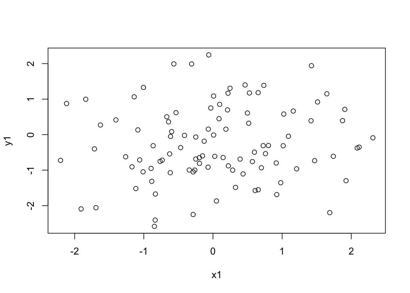
Figure 2.1: A basic scatterplot
plot(x1,y1,pch=16, col='red')x2 <- seq(0,2*pi,len=100)
y2 <- sin(x2)plot(x2,y2,type='l')
plot(x2,y2,type='l', lwd=3, col='darkgreen') plot(x2,y2,type='l', col='darkgreen', lwd=3, ylim=c(-1.2,1.2))
y2r <- y2 + rnorm(100,0,0.1)
points(x2,y2r, pch=16, col='darkred')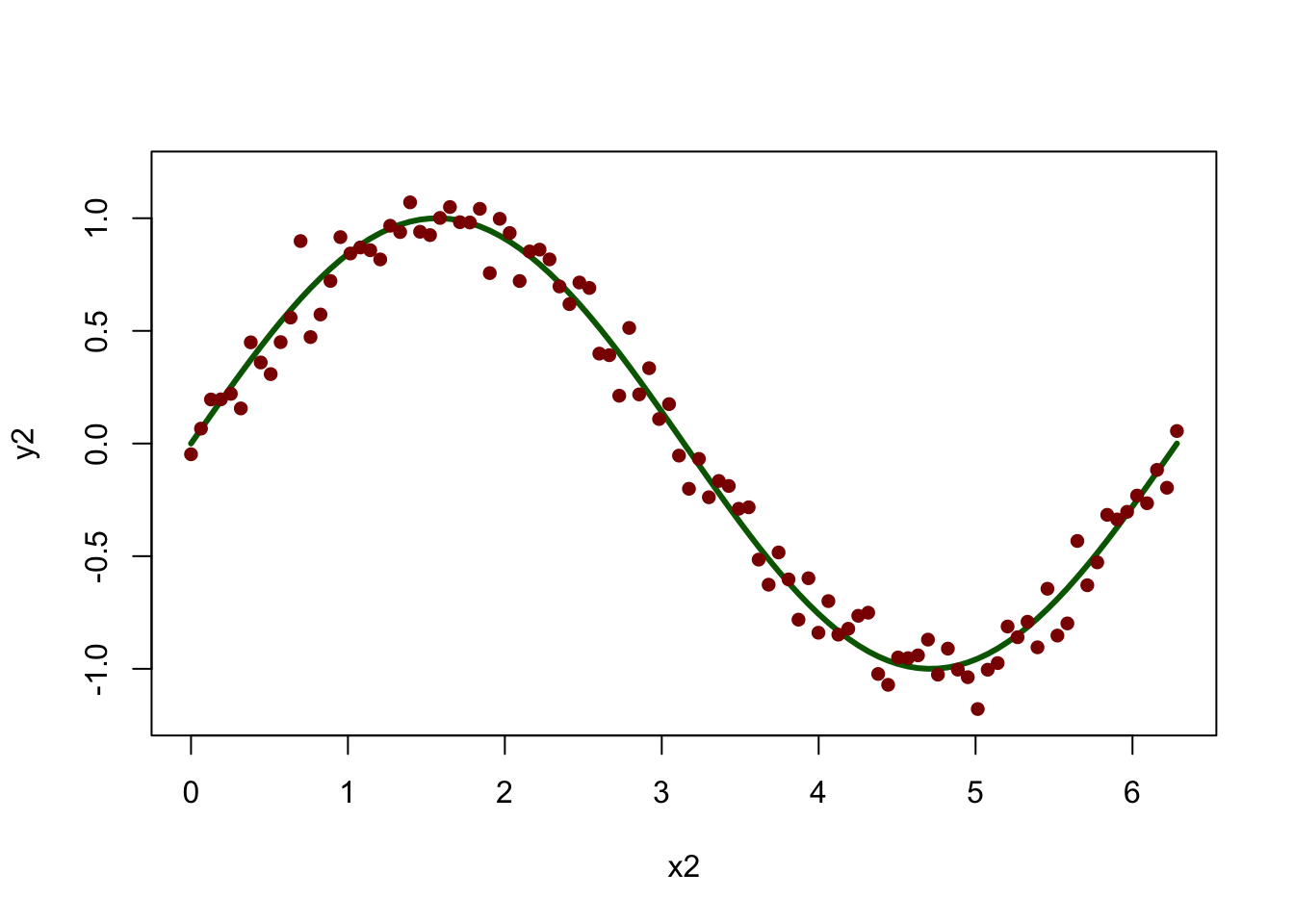
Figure 2.2: A line plot with points added
y4 <- cos(x2)
plot(x2, y2, type='l', lwd=3, col='darkgreen')
lines(x2, y4, lwd=3, lty=2, col='darkblue')
x2 <- seq(0,2*pi,len=100)
y2 <- sin(x2)
y4 <- cos(x2)
# specify the plot layout and order
par(mfrow = c(1,2))
# plot #1
plot(y2,y4)
polygon(y2,y4,col='lightgreen')
# plot #2: this time with 'asp' to set the aspect ratio of the axes
plot(y2,y4, asp=1, type='n')
polygon(y2,y4,col='lightgreen')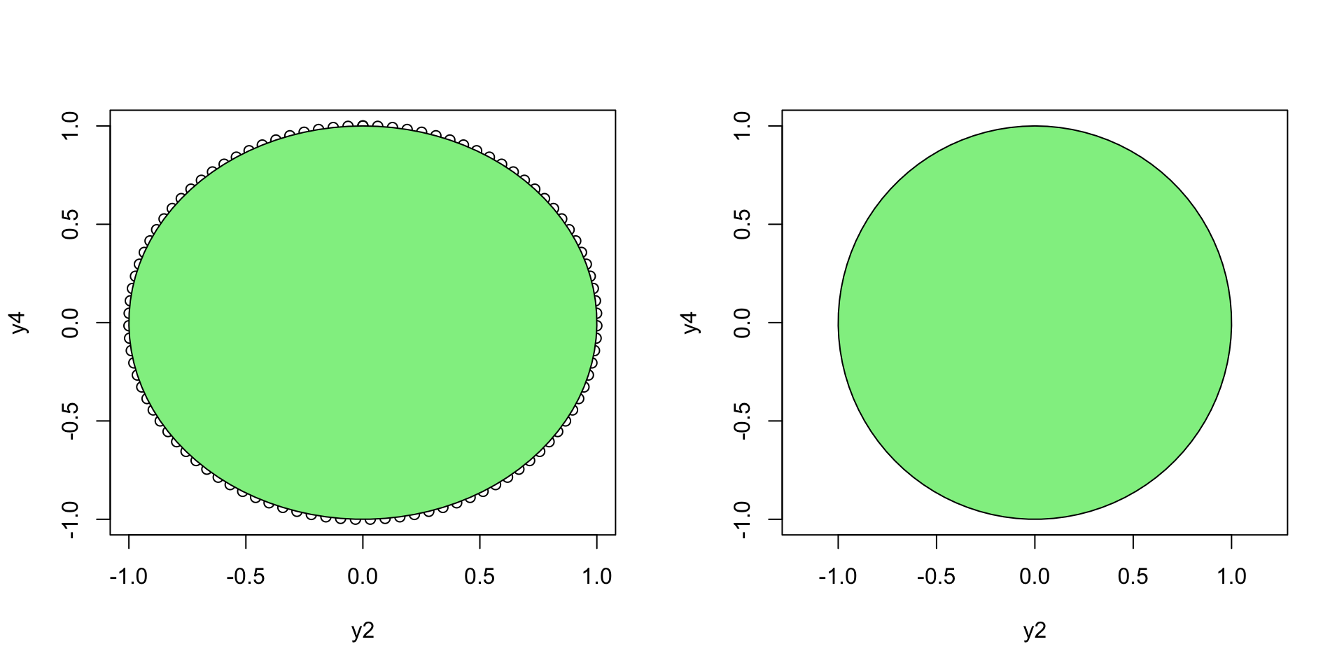
Figure 2.3: Points with polygons added
Addendum September 2022: The GISTools package is in the process of being updated. To install it as a temporary fix, there are 2 options:
- Run the code below.
# Download package tarball from CRAN archive
url <- "https://cran.r-project.org/src/contrib/Archive/GISTools/GISTools_0.7-4.tar.gz"
pkgFile <- "GISTools_0.7-4.tar.gz"
download.file(url = url, destfile = pkgFile)

# Install dependencies list in the DESCRIPTION file
install.packages(c("maptools", "sp", "RColorBrewer", "MASS", "rgeos"))

# Install package
install.packages(pkgs=pkgFile, type="source", repos=NULL)

# Delete package tarball
unlink(pkgFile)

# Load the package
library(GISTools)- Or, if you get install errors due to your computer environment (e.g. Microsoft Windows with UNC paths) do this manually.
- Install dependencies listed in the DESCRIPTION file
install.packages(c("maptools", "sp", "RColorBrewer", "MASS", "rgeos"))Manually download ‘GISTools_0.7-4.tar.gz’ from https://cran.r-project.org/src/contrib/Archive/GISTools/
In RStudio go to Tools > Install Packages > Install from select “Package Archive File (.zip; .tar.gz)” then browse and select the manually downloaded ‘GISTools_0.7-4.tar.gz’ and then select Install
Load the package
library(GISTools)# library(GISTools)
data(georgia)
# select the first element
appling <- georgia.polys[[1]]
# set the plot extent
plot(appling, asp=1, type='n', xlab="Easting", ylab="Northing")
# plot the selected features with hatching
polygon(appling, density=14, angle=135) 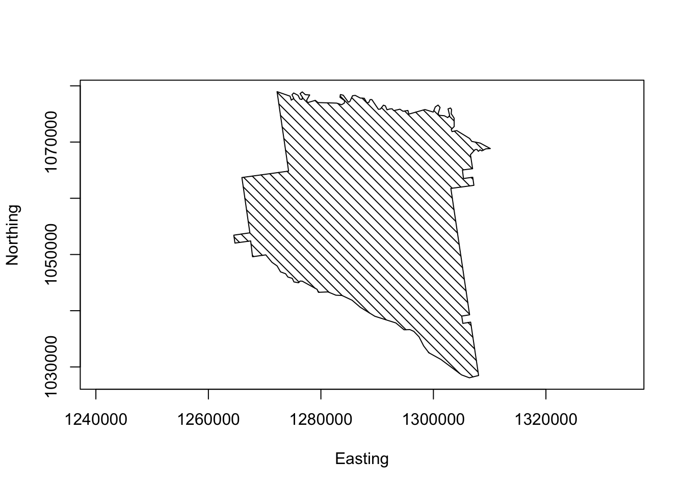
Figure 2.4: Appling County plotted from coordinate pairs
2.4.2 Plot colours
colours()plot(appling, asp=1, type='n', xlab="Easting", ylab="Northing")
polygon(appling, col=rgb(0,0.5,0.7))polygon(appling, col=rgb(0,0.5,0.7,0.4))# set the plot extent
plot(appling, asp=1, type='n', xlab="Easting", ylab="Northing")
# plot the points
points(x = runif(500,126,132)*10000,
y = runif(500,103,108)*10000, pch=16, col='red')
# plot the polygon with a transparency factor
polygon(appling, col=rgb(0,0.5,0.7,0.4))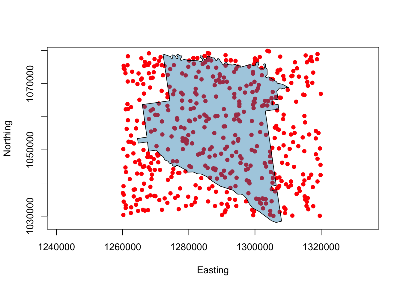
Figure 2.5: Appling County with transparency
plot(appling, asp=1, type='n', xlab="Easting", ylab="Northing")
polygon(appling, col="#B3B333")
# add text, sepcifying its placement, colour and size
text(1287000,1053000,"Appling County",cex=1.5)
text(1287000,1049000,"Georgia",col='darkred')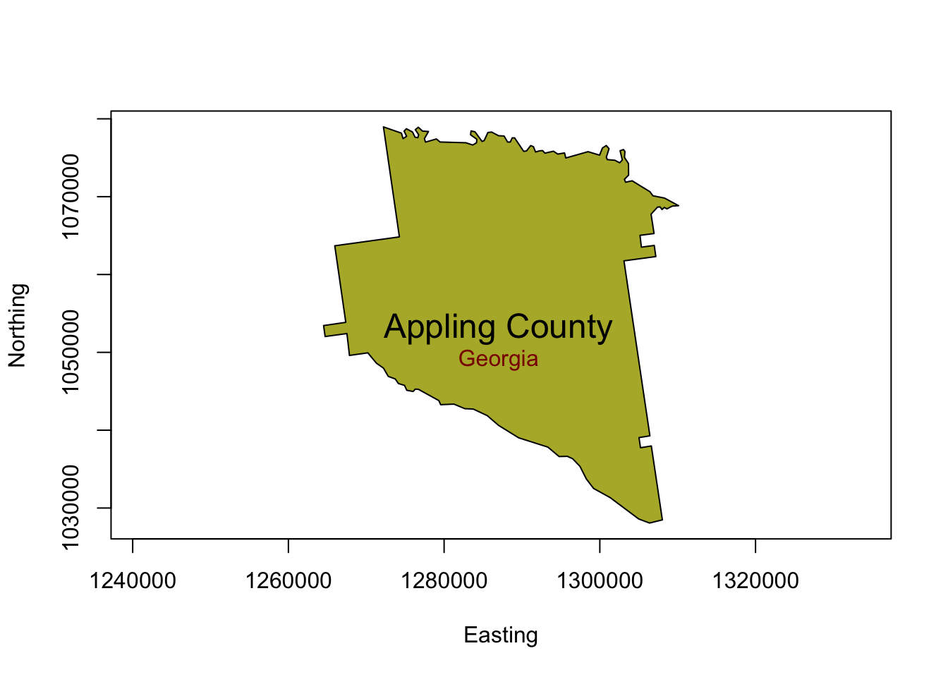
Figure 2.6: Appling County with text
plot(c(-1.5,1.5),c(-1.5,1.5),asp=1, type='n')
# plot the green/blue rectangle
rect(-0.5,-0.5,0.5,0.5, border=NA, col=rgb(0,0.5,0.5,0.7))
# then the second one
rect(0,0,1,1, col=rgb(1,0.5,0.5,0.7))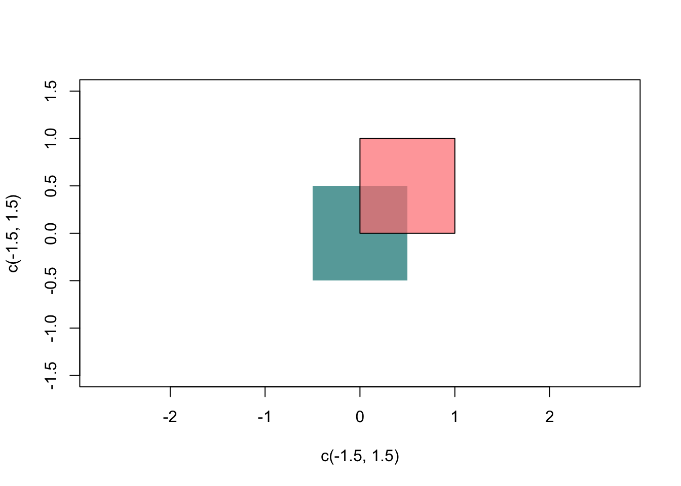
Figure 2.7: Plotting rectangles
# load some grid data
data(meuse.grid)
# define a SpatialPixelsDataFrame from the data
mat = SpatialPixelsDataFrame(points = meuse.grid[c("x", "y")],
    data = meuse.grid)
# set some plot parameters (1 row, 2 columns)
par(mfrow = c(1,2))
# set the plot margins
par(mar = c(0,0,0,0))
# plot the points using the default shading
image(mat, "dist")
# load the package
library(RColorBrewer)
# select and examine a colour palette with 7 classes
greenpal <- brewer.pal(7,'Greens')
# and now use this to plot the data
image(mat, "dist", col=greenpal)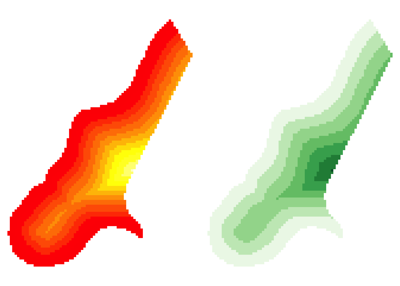
Figure 2.8: Plotting raster data
# reset par
par(mfrow = c(1,1))
2.5 Another plot option: ggplot
2.5.1 Introduction to ggplot
install.packages("tidyverse", dep = T)install.packages("ggplot2", dep = T)library(ggplot2)qplot(x2,y2r,col=I('darkred'), ylim=c(-1.2, 1.2)) +
geom_line(aes(x2,y2), col=I("darkgreen"), size = I(1.5)) +
theme(axis.text=element_text(size=20),
axis.title=element_text(size=20,face="bold"))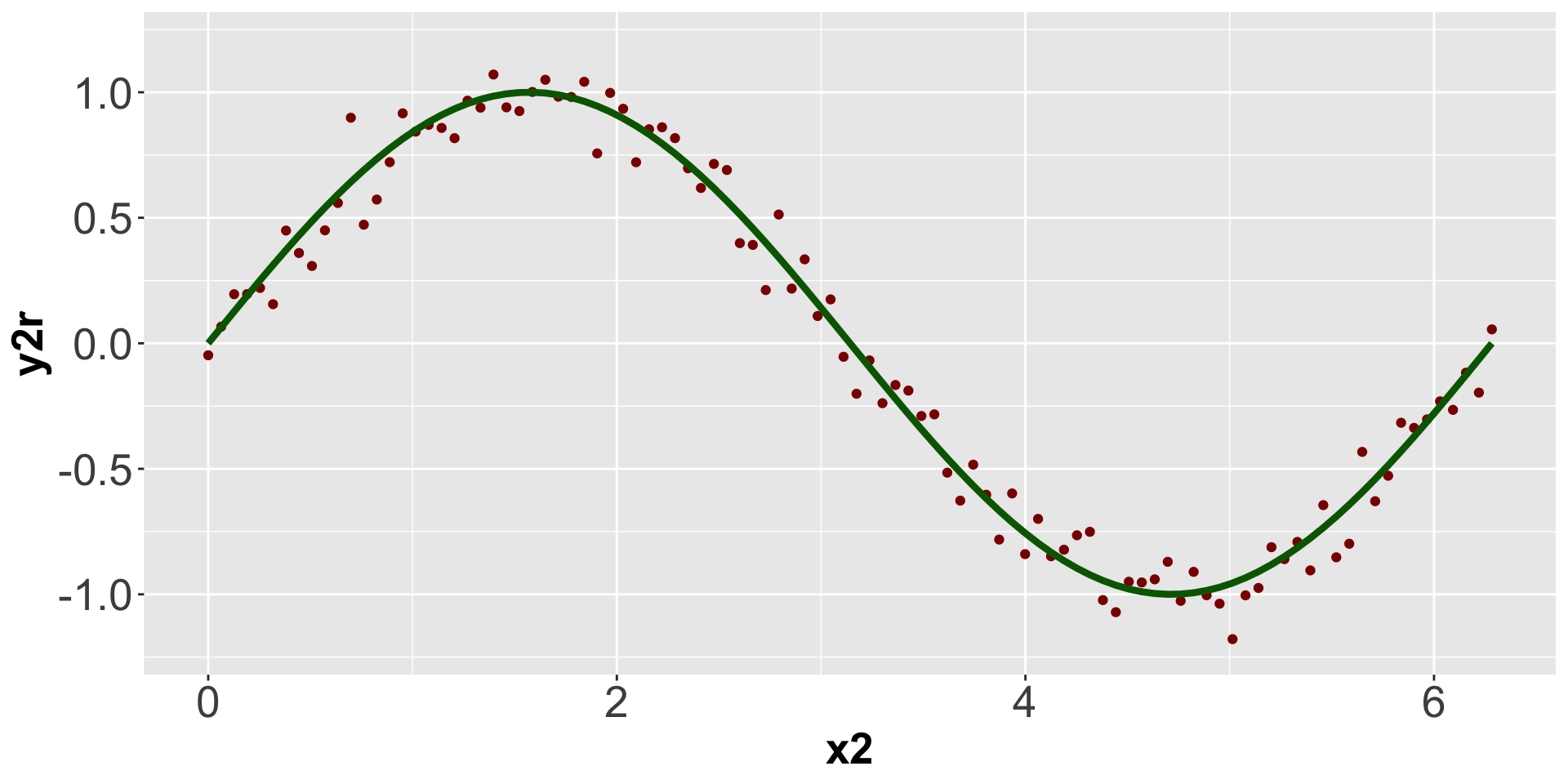
Figure 2.9: A simple qplot
theme_bw() theme_dark()appling <- data.frame(appling)
colnames(appling) <- c("X", "Y")install.packages("gridExtra", dep = T)# create the first plot with qplot
p1 <- qplot(X, Y, data = appling, geom = "polygon", asp = 1,
colour = I("black"),
fill=I(rgb(0,0.5,0.7,0.4))) +
theme(axis.text=element_text(size=12),
axis.title=element_text(size=20))
# create a data.frame to hold the points
df <- data.frame(x = runif(500,126,132)*10000,
y = runif(500,103,108)*10000)
# now use ggplot to contruct the layers of the plot
p2 <- ggplot(appling, aes(x = X, y= Y)) +
geom_polygon(fill = I(rgb(0,0.5,0.7,0.4))) +
geom_point(data = df, aes(x, y),col=I('red')) +
coord_fixed() +
theme(axis.text=element_text(size=12),
axis.title=element_text(size=20))
# finally combine these in a single plot
# using the grid.arrange function
# NB you may have to install the gridExtra package
library(gridExtra)
grid.arrange(p1, p2, ncol = 2)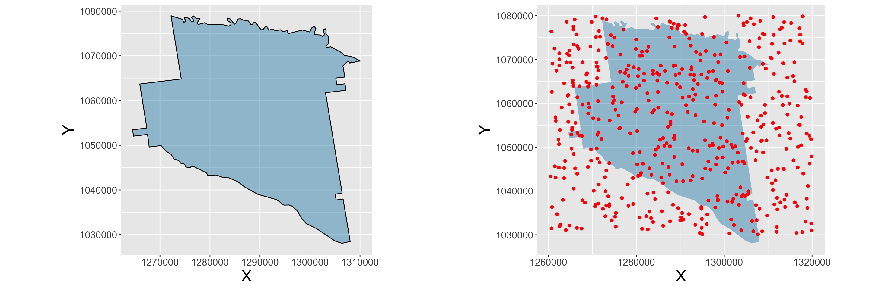
Figure 2.10: A simple qplot of a polygon
2.5.2 Different ggplot types
# data.frame
df <- data.frame(georgia)
# tibble
tb <- as.tibble(df)tbtb$rural <- as.factor((tb$PctRural > 50) + 0)
levels(tb$rural) <- list("Non-Rural" = 0, "Rural"=1)tb$IncClass <- rep("Average", nrow(tb))
tb$IncClass[tb$MedInc >= 41204] = "Rich"
tb$IncClass[tb$MedInc <= 29773] = "Poor"table(tb$IncClass)ggplot(data = tb, mapping=aes(x=PctBach, y=PctEld)) +
geom_point()ggplot(data = tb, mapping=aes(x=PctBach, y=PctEld, colour=rural)) +
geom_point()ggplot(data = tb, mapping = aes(x = PctBach, y = PctEld)) +
geom_point() +
geom_smooth(method = "lm")ggplot(data = tb, mapping = aes(x = PctBach, y = PctEld)) +
geom_point() +
geom_smooth(method = "lm", col = "red", fill = "lightsalmon") +
theme_bw() +
xlab("% of population with bachelor degree") +
ylab("% of population that are elderly") 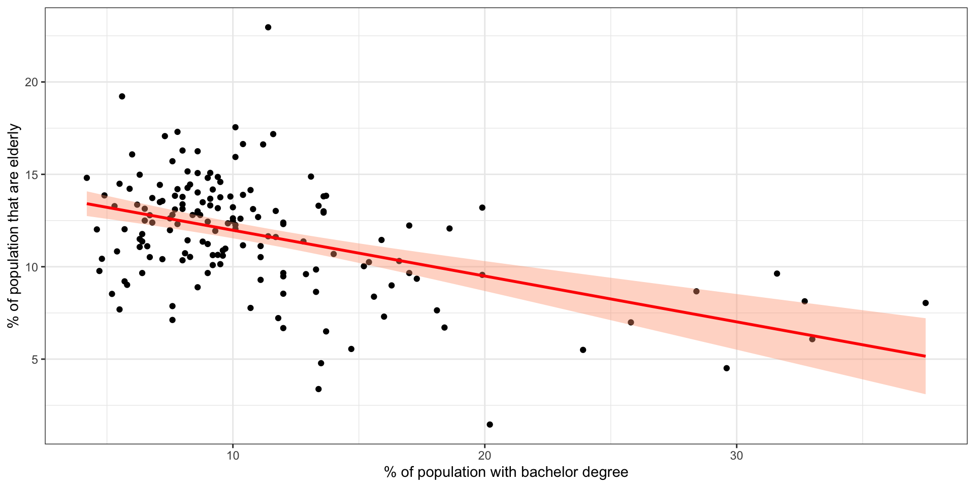
Figure 2.11: A ggplot scatterplot
ggplot(tb, aes(x=MedInc)) +
geom_histogram(, binwidth = 5000, colour = "red", fill = "grey")ggplot(tb, aes(x=MedInc)) +
geom_histogram(aes(y=..density..),
binwidth=5000,colour="white") +
geom_density(alpha=.4, fill="darksalmon") +
# Ignore NA values for mean
geom_vline(aes(xintercept=median(MedInc, na.rm=T)),
color="orangered1", linetype="dashed", size=1)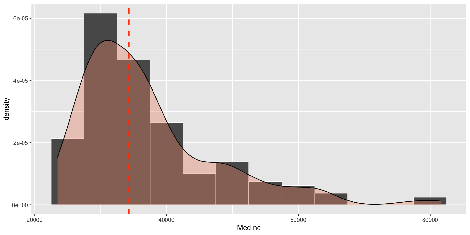
Figure 2.12: A ggplot density histogram
ggplot(tb, aes(x=PctBach, fill=IncClass)) +
  geom_histogram(color="grey30",
    binwidth = 1) +
    scale_fill_manual("Income Class",
    values = c("orange", "palegoldenrod","firebrick3")) +
  facet_grid(IncClass~.) +
  xlab("% Bachelor degrees") +
ggtitle("Bachelors degree % in different income classes")gplot(tb, aes(x = "",PctBach)) +
geom_boxplot() ggplot(tb, aes(IncClass, PctBach, fill = factor(rural))) +
geom_boxplot() +
scale_fill_manual(name = "Rural",
values = c("orange", "firebrick3"),
labels = c("Non-Rural"="Not Rural","Rural"="Rural")) +
xlab("Income Class") +
ylab("% Bachelors")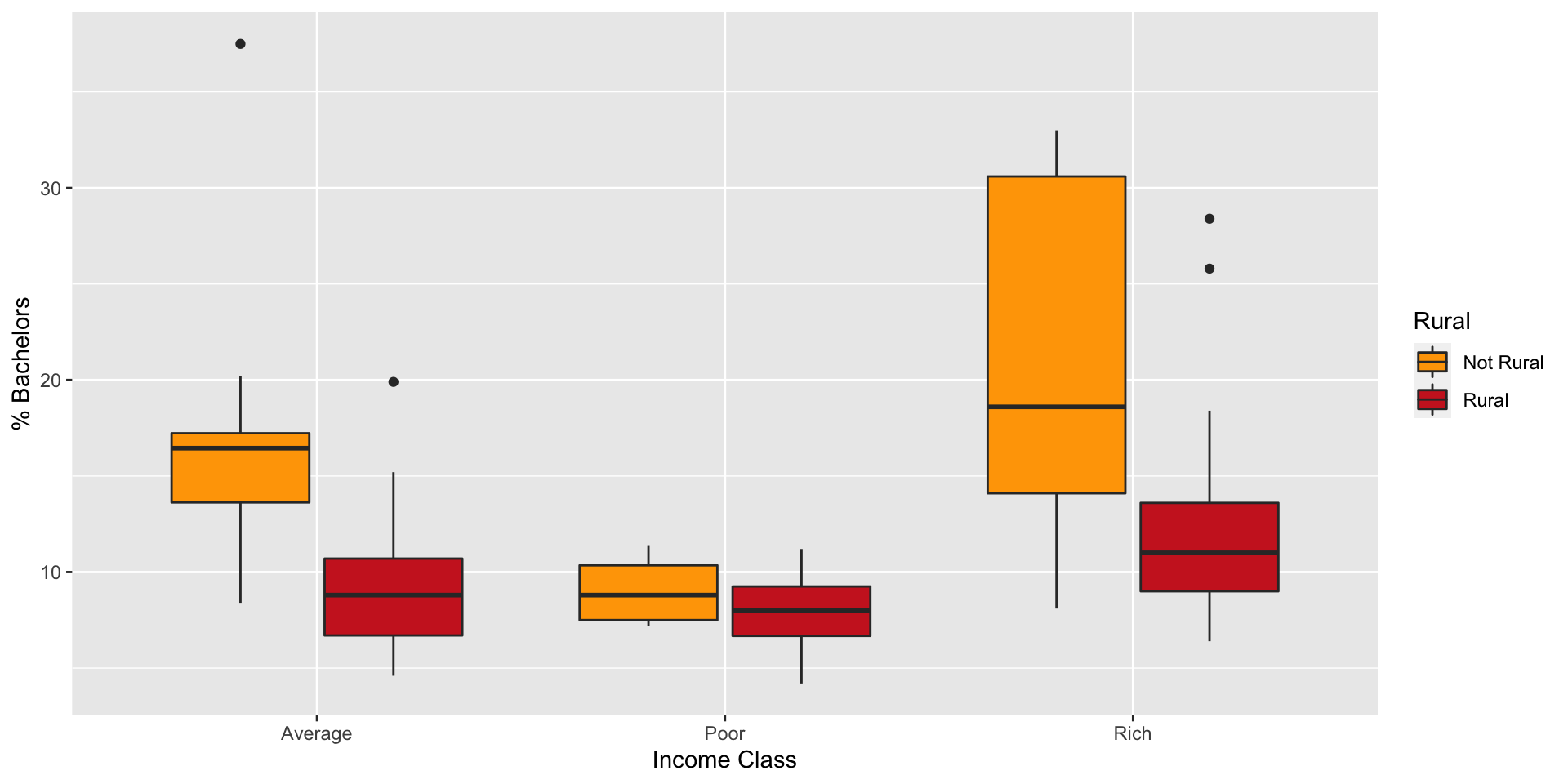
Figure 2.13: A ggplot boxplot with groups
2.6 Reading, writing, loading and saving data
2.6.1 Text files
# display the first six rows
head(appling)
# display the variable dimensions
dim(appling)colnames(appling) <- c("X", "Y")write.csv(appling, file = "test.csv")write.csv(appling, file = "test.csv", row.names = F)tmp.appling <- read.csv(file = "test.csv")2.6.2 R Data files
# this will save everything in the workspace
save(list = ls(), file = "MyData.RData")
# this will save just appling
save(list = "appling", file = "MyData.RData")
# this will save appling and georgia.polys
save(list = c("appling", "georgia.polys"), file = "MyData.RData")load("MyData.RData")2.6.3 Spatial Data files
library(rgdal)writeOGR(obj=georgia, dsn=".", layer="georgia",
driver="ESRI Shapefile", overwrite_layer=T) new.georgia <- readOGR("georgia.shp") install.packages("sf", dep = T)
library(sf)
setwd("/MyPath/MyFolder")
g2 <- st_read("georgia.shp")
st_write(g2, "georgia.shp", delete_layer = T)2.7 Answers to self-test questions
Q1
colours[4] <- "orange"
colours
[1] red blue red <NA> silver red white silver
[9] red red white silver silver
Levels: red blue white silver blackQ2
Q3
Q4
# Undo the colour[4] <- 'orange' line used above
colours <- factor(c("red","blue","red","white","
    silver","red","white","silver",
    "red","red","white","silver"),
 levels=c("red","blue","white","silver","black"))
colours[engine > "1.1litre"]
[1] blue white <NA> red white red silver <NA>
Levels: red blue white silver blacktable(car.type[engine < "1.6litre"])
     saloon   hatchback convertible
7 4 0 table(colours[(engine >= "1.3litre") & (car.type == "hatchback")])
   red   blue  white silver  black
     2      0      0      0      0
Q5
Q6
apply(crosstab,1,which.max) saloon hatchback convertible
1 1 3 Q7
apply(crosstab,1,which.max.name) saloon hatchback convertible
"red" "red" "white" apply(crosstab,2,which.max.name) red blue white silver black
"hatchback" "saloon" "saloon" "saloon" "saloon" Q8
most.popular <- list(colour=apply(crosstab,1,which.max.name),
type=apply(crosstab,2,which.max.name))
most.popular$colour
     saloon   hatchback convertible
      "red"       "red"     "white"
$type
        red        blue       white      silver       black
"hatchback" "saloon" "saloon" "saloon" "saloon" Q9
print.sales.data <- function(x) {
  cat("Weekly Sales Data:\n")
  cat("Most popular colour:\n")
  for (i in 1:length(x$colour)) {
    cat(sprintf("%12s:%12s\n",names(x$colour)[i],x$colour[i]))}
  cat("Most popular type:\n")
  for (i in 1:length(x$type)) {
    cat(sprintf("%12s:%12s\n",names(x$type)[i],x$type[i]))}
  cat("Total Sold = ",x$total)
}