Chapter 4 Scripting and Writing Functions in R

4.1 Overview

4.2 Introduction

tree.heights <- c(4.3,7.1,6.3,5.2,3.2)

tree.heights

[1] 4.3 7.1 6.3 5.2 3.2

if (tree.heights[1] < 6) { cat('Tree is small\n') } else 
  { cat('Tree is large\n')} 

Tree is small

for(variable in sequence) R expression

for (i in 1:3) {
    if (tree.heights[i] < 6) { cat('Tree',i,' is small\n') } 
    else { cat('Tree',i,' is large\n')} }

Tree 1  is small
Tree 2  is large
Tree 3  is large

assess.tree.height <- function(tree.list, thresh) 
  { for (i in 1:length(tree.list))
    { if(tree.list[i] < thresh) {cat('Tree',i, ' is small\n')}
      else { cat('Tree',i,' is large\n')} 
    }
  }
assess.tree.height(tree.heights, 6)

Tree 1  is small
Tree 2  is large
Tree 3  is large
Tree 4  is small
Tree 5  is small

tree.heights2 <- c(8,4.5,6.7,2,4)
assess.tree.height(tree.heights2, 4.5)

Tree 1  is large
Tree 2  is large
Tree 3  is large
Tree 4  is small
Tree 5  is small

4.3 Building blocks for Programs

4.3.1 Conditional Statements

x <- -7
if (x < 0) cat("x is negative")

x is negative

x <- 8
if (x < 0) cat("x is negative")

x <- -7
if (x < 0) cat("x is negative") else cat("x is positive")

x is negative

x <- 8
if (x < 0) cat("x is negative") else cat("x is positive")

x is positive

??is.

x <- c(1,3,6,8,9,5)
if (all(x > 0)) cat("All numbers are positive") 

All numbers are positive

x <- c(1,3,6,-8,9,5)
if (any(x > 0)) cat("Some numbers are positive") 

Some numbers are positive

any(x==0)

[1] FALSE

4.3.2 Code Blocks: \(\{\) and \(\}\)

x <- c(1,3,6,8,9,5)
if (all(x > 0)) {
  cat("All numbers are positive\n") 
  total <- sum(x)
  cat("Their sum is ",total) }

All numbers are positive
Their sum is  32

if condition { consequents }  else { alternatives }

x <- c(1,3,6,8,9,-5)
if (all(x > 0)) {
  cat("All numbers are positive\n") 
  total <- sum(x)
  cat("Their sum is ",total) }  else {
  cat("Not all numbers are positive\n")
  cat("This is probably an error as numbers are rainfall levels") }

Not all numbers are positive
This is probably an error as numbers are rainfall levels

4.3.3 Functions

mean.rainfall <- function(rf)  
{ if (all(rf> 0))                 #open Function
  { mean.value <- mean(rf)        #open Consequent
    cat("The mean is ",mean.value) 
  } else                          #close Consequent
    { cat("Warning: Not all values are positive\n")  #open Alternative
    }                             #close Alternative
  }                               #close Function
mean.rainfall(c(8.5,9.3,6.5,9.3,9.4))  

The mean is  8.6

mean.rainfall2 <- function(rf) {
if (all(rf> 0)) {
  return( mean(rf))} else {
  return(NA)}
  }
mr <- mean.rainfall2(c(8.5,9.3,6.5,9.3,9.4))  
mr

[1] 8.6

rf <- "Tuesday"
mean.rainfall2(c(8.5,9.3,6.5,9.3,9.4))  

[1] 8.6

rf

[1] "Tuesday"

4.3.4 Loops and repetition

for (i in 1:5) {
    i.cubed <- i * i * i
    cat("The cube of",i,"is ",i.cubed,"\n")}

The cube of 1 is  1 
The cube of 2 is  8 
The cube of 3 is  27 
The cube of 4 is  64 
The cube of 5 is  125 

seq(from, to, by = step value)

seq(from, to, length = sequence length)

for (val in seq(0,1,by=0.25)) {
    val.squared <- val * val 
    cat("The square of",val,"is ",val.squared,"\n")}

The square of 0 is  0 
The square of 0.25 is  0.0625 
The square of 0.5 is  0.25 
The square of 0.75 is  0.5625 
The square of 1 is  1 

i <- 1; n <- 654
repeat{
  i.squared <- i * i
  if (i.squared > n) break
  i <- i + 1}
cat("The first square number exceeding",n, "is ",i.squared,"\n")

The first square number exceeding 654 is  676 

first.bigger.square <- function(n) {
    i <- 1
    repeat{
        i.squared <- i * i
        if (i.squared > n) break
        i <- i + 1 }
    return(i.squared)}

first.bigger.square(76987)

[1] 77284

4.3.5 Debugging

4.4 Writing Functions

4.4.1 Introduction

cube.root <- function(x) {
   result <- x ^ (1/3)
   return(result)}
cube.root(27)

[1] 3

source("functions.R")

cube.root <- function(x) { 
    result <- x ^ (1/3) 
    return(result)} 

source('functions.R')
cube.root(343)
cube.root(99)

circle.area <- function(r) { 
    result <- pi * r ^ 2
    return(result)} 

source('functions.R')
cube.root(343)
circle.area(10)

4.4.2 Data Checking

cube.root(-343)

[1] NaN

cube.root <- function(x) {
    if (x >= 0) { 
       result <- x ^ (1/3) }  else {
       result <- -(-x) ^ (1/3) }
    return(result)} 

cube.root(3)

[1] 1.44225

cube.root(-3)

[1] -1.44225

debug(cube.root)

cube.root(-50)

x > 0

undebug(cube.root)

help(debug)

4.4.3 More Data Checking

cube.root('Leeds')

is.numeric(77)
is.numeric("Lex")
is.numeric("77")
v <- "Two Sevens Clash"
is.numeric(v)

cube.root <- function(x) { 
  if (is.numeric(x)) { 
    if (x >= 0) { result <- x^(1/3) }  
    else { result <- -(-x)^(1/3) }
    return(result) }  
  else { 
    cat("WARNING: Input must be numerical, not character\n") 
    return(NA)}
  }

4.4.4 Loops Revisited

4.4.4.1 Conditional Loops

gcd <- function(a,b)
  {
     divisor <- min(a,b)
     dividend <- max(a,b)
     repeat 
       { remainder <- dividend %% divisor
         dividend <- divisor
         divisor <- remainder
         if (remainder == 0) break
        }
     return(dividend)
 }

gcd(6,15)
gcd(25,75)
gcd(31,33)

4.4.4.2 Deterministic Loops

cube.root.table <- function(n)
  {
    for (x in 1:n) 
    {
      cat("The cube root of ",x," is", cube.root(x),"\n")
    }
  }

4.4.5 Further Activity

cat(sprintf("The cube root of %4.0f is %8.4f \n",x,cube.root(x)))

library(GISTools)
library(sf)
data(georgia)
# create an empty list for the results
adj.list <- list()
# convert georgia to sf 
georgia_sf <- st_as_sf(georgia2)
# extract a single county
county.i <- georgia_sf[1,]
# determine the adjacent counties
# the [-1] removes Appling form its own list
adj.i <- unlist(st_intersects(county.i, georgia_sf))[-1]
# extract their names
adj.names.i <- georgia2$Name[adj.i]
# add to the list
adj.list[[1]] <- adj.i
# name the list elements
names(adj.list[[1]]) <- adj.names.i

adj.list

[[1]]
     Bacon Jeff Davis     Pierce   Tattnall     Toombs 
         3         80        113        132        138 
     Wayne 
       151 

# in sequence 
adj.list[[2]] <- sample(1:100, 3)
# or not!
i = 4
adj.list[[i]] <- c("Chris", "and", "Lex")
# have a look!
adj.list

4.5 Spatial data structures

rm(list = ls())

library(GISTools)
data(georgia)

ls()

georgia.polys

class(georgia.polys)

[1] "list"

head(georgia.polys[[1]])

        [,1]    [,2]
[1,] 1292287 1075896
[2,] 1292654 1075919
[3,] 1292949 1075590
[4,] 1294045 1075841
[5,] 1294603 1075472
[6,] 1295467 1075621

.

# plot Appling
plot(georgia.polys[[1]],asp=1,type='l',
     xlab = "Easting", ylab = "Northing")
# plot adjacent county outlines
points(georgia.polys[[3]],asp=1,type='l', col = "red")
points(georgia.polys[[151]],asp=1,type='l', col = "blue", lty = 2)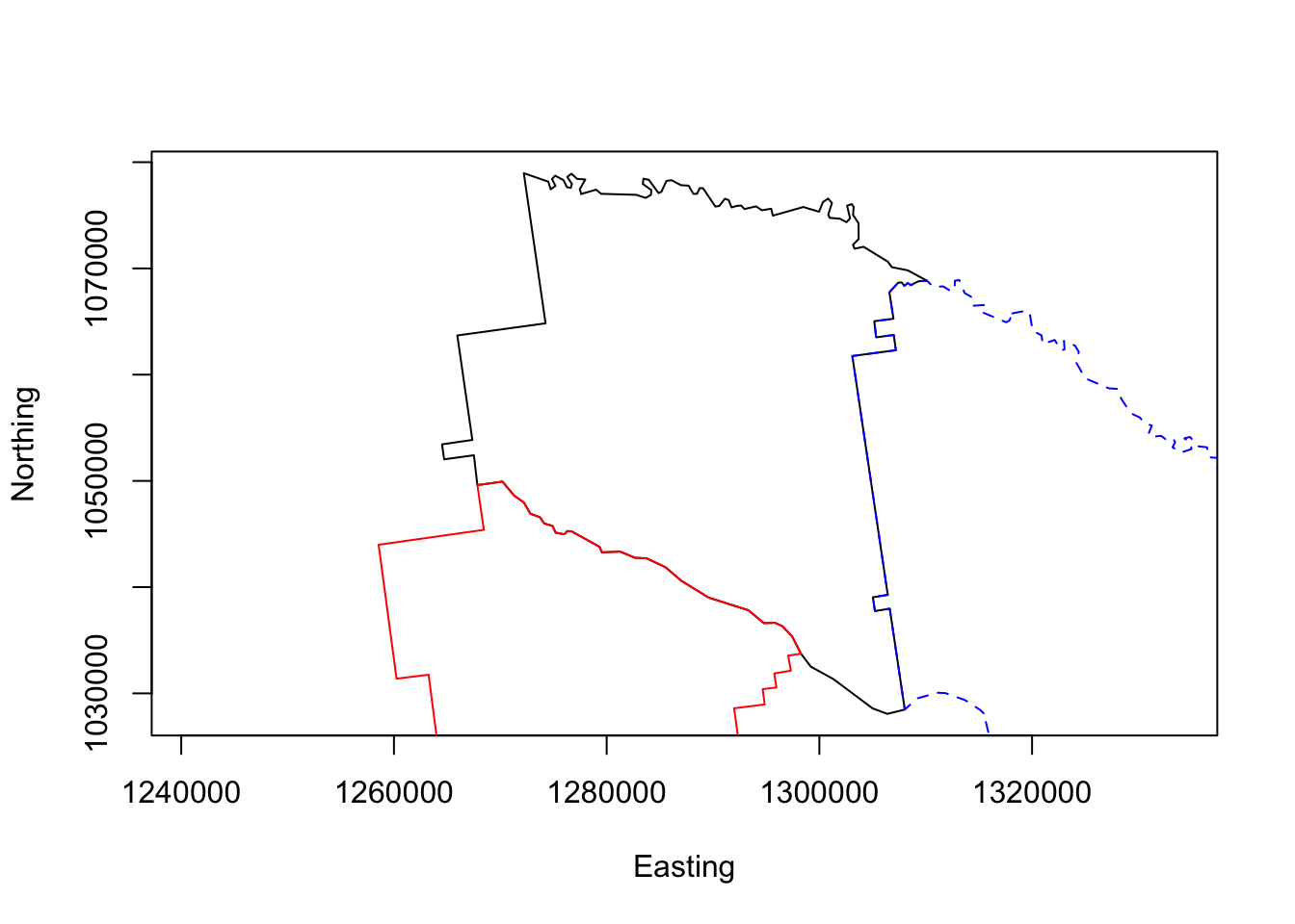

Figure 4.1: A simple plot of Appling County and 2 adjacent counties.

head(georgia2@polygons[[1]]@Polygons[[1]]@coords)
head(georgia2@data[, 13:14])

g <- st_as_sf(georgia2)
head(g[,13:14])

4.6 Apply functions

library(GISTools)
data(newhaven)
## the @data route
head(blocks@data[, 14:17])
## the data frame route
head(data.frame(blocks[, 14:17]))

apply(blocks@data[,14:17], 1, max)

apply(blocks@data[,14:17], 2, max)

# set up vector to hold result
result.vector <- vector()
for (i in 1:nrow(blocks@data)){
  # for each row determine which column has the max value
  result.i <- which.max(data.frame(blocks[i,14:17]))
  # put into the result vector
  result.vector <- append(result.vector, result.i)
}

res.vec <-apply(data.frame(blocks[,14:17]), 1, which.max)
# comapre the two results
identical(as.vector(res.vec), as.vector(result.vector))

# Loop
t1 <- Sys.time()
result.vector <- vector()
for (i in 1:nrow(blocks@data)){
  result.i <- which.max(data.frame(blocks[i,14:17]))
  result.vector <- append(result.vector, result.i)
}
Sys.time() - t1
# Apply
t1 <- Sys.time()
res.vec <-apply(data.frame(blocks[,14:17]), 1, which.max)
Sys.time() - t1

plot(bbox(georgia2)[1,], bbox(georgia2)[2,], asp = 1, 
     type='n',xlab='',ylab='',xaxt='n',yaxt='n',bty='n')
for (i in 1:length(georgia.polys)){
  points(georgia.polys[[i]], type='l')
  # small delay so that you can see the plotting
  Sys.sleep(0.05)
}

plot(bbox(georgia2)[1,], bbox(georgia2)[2,], asp = 1, 
     type='n',xlab='',ylab='',xaxt='n',yaxt='n',bty='n')
invisible(mapply(polygon,georgia.polys))

# create a distance matrix
dMat <- as.matrix(dist(coordinates(georgia2)))
dim(dMat)
# create an empty vector
count.vec <- vector()
# create an empty list
names.list <- list()
# for each county...
for( i in 1:nrow(georgia_sf)) {
  # which counties are within 50km
  vec.i <- which(dMat[i,] <= 50000)
  # add to the vector
  count.vec <- append(count.vec, length(vec.i))
  # find their names
  names.i <- georgia_sf$Name[vec.i]
  # add to the list
  names.list[[i]] <- names.i
}
# have a look! 
count.vec
names.list

lapply(names.list, length)

count.vec <- apply(dMat,1.my.func1)
names.list <- apply(dMat,1.my.func2)

4.7 Manipulating data with dplyr

vignette("introduction", package = "dplyr")

install.packages("nycflights13")
library("nycflights13")
class(flights)
flights

data(package = "nycflights13")

vignette("two-table", package = "dplyr")

flights2 <- flights %>% select(year:day,hour,origin,dest,tailnum,carrier)

flights2 <- select(flights, year:day,hour,origin,dest,tailnum,carrier)

library(nycflights13)
library(tidyverse)
# select the variables
flights2 <- flights %>% select(origin, dest)
# remove Alaska and Hawaii
flights2 <- flights2[-grep("ANC", flights2$dest),]
flights2 <- flights2[-grep("HNL", flights2$dest),]
# group by destination
flights2 <- group_by(flights2, dest) 
flights2 <- summarize(flights2, count = n())
# assign Lat and Lon for Origin
flights2$OrLat <- 40.6925 
flights2$OrLon <- -74.16867
# have a look! 
flights2

# A tibble: 103 x 4
   dest  count OrLat OrLon
   <chr> <int> <dbl> <dbl>
 1 ABQ     254  40.7 -74.2
 2 ACK     265  40.7 -74.2
 3 ALB     439  40.7 -74.2
 4 ATL   17215  40.7 -74.2
 5 AUS    2439  40.7 -74.2
 6 AVL     275  40.7 -74.2
 7 BDL     443  40.7 -74.2
 8 BGR     375  40.7 -74.2
 9 BHM     297  40.7 -74.2
10 BNA    6333  40.7 -74.2
# ... with 93 more rows

library(maps)
library(geosphere)
# origin and desitnation examples
dest.eg <- matrix(c(77.1025, 28.7041), ncol = 2)
origin.eg <- matrix(c(-74.16867, 40.6925), ncol = 2)
# map the world from the maps package data
map("world", fill=TRUE, col="white", bg="lightblue")
# plot the points
points(dest.eg, col="red", pch=16, cex = 2)
points(origin.eg, col = "cyan", pch = 16, cex = 2)
# add the route
for (i in 1:nrow(dest.eg)) {
    lines(gcIntermediate(dest.eg[i,], origin.eg[i,], n=50, 
        breakAtDateLine=FALSE, addStartEnd=FALSE, 
        sp=FALSE, sepNA), lwd = 2, lty = 2)
}

map("usa", fill=TRUE, col="white", bg="lightblue")

4.8 Answers to self-test questions

Q1

cube.root.2 <- function(x) 
 { if (is.numeric(x)) 
   { result <- sign(x)*abs(x)^(1/3)
      return(result)  
   } else
 { cat("WARNING: Input must be numerical, not character\n") 
   return(NA) }
}

Q2

gcd <- function(a,b)
  {
     divisor <- min(a,b) # line 1
     dividend <- max(a,b) # line 1
     repeat #line 5
       { remainder <- dividend %% divisor #line 2
         dividend <- divisor # line 3
         divisor <- remainder # line 4
         if (remainder == 0) break #line 6 
        }
     return(dividend)
 }

Q3 part i)

gcd.60 <- function(a)
  {
    for(i in 1:a) 
    { divisor <- min(i,60)
       dividend <- max(i,60)
        repeat 
        { remainder <- dividend %% divisor
            dividend <- divisor
            divisor <- remainder
            if (remainder == 0) break
         }
      cat(dividend, "\n")   
     }
  }

gcd.60 <- function(a)
  {  for(i in 1:a) 
    { dividend <- gcd(i,60)
      cat(i,":", dividend, "\n")    
    }
  }

Q3 part ii)

gcd.all <- function(x,y)
  {  for(n1 in 1:x) 
    {  for (n2 in 1:y) 
        { dividend <- gcd(n1, n2)
          cat("when x is",n1,"& y is",n2,"dividend =",dividend,"\n")
            }
     }
  }

Q4

cube.root.table <- function(n)
  { for (x in seq(0.5, n, by = 0.5)) 
    { cat("The cube root of ",x," is", 
          sign(x)*abs(x)^(1/3),"\n")  }
  }

cube.root.table <- function(n)
  { if (n < 0 ) by.val = 0.5
    if (n < 0 ) by.val =-0.5
    for (x in seq(0.5, n, by = by.val)) 
    { cat("The cube root of ",x," is", 
      sign(x)*abs(x)^(1/3),"\n") }
  }

Q5

# create an empty list for the results
adj.list <- list()
# convert georgia to sf 
georgia_sf <- st_as_sf(georgia2)
for (i in 1:nrow(georgia_sf)) {
  # extract a single county
  county.i <- georgia_sf[i,]
  # determine the adjacent counties
  # the [-1] removes Appling form its own list
  adj.i <- unlist(st_intersects(county.i, georgia_sf))[-1]
  # extract their names
  adj.names.i <- georgia2$Name[adj.i]
  # add to the list
  adj.list[[i]] <- adj.i
  # name the list elements
  names(adj.list[[i]]) <- adj.names.i
}

Q6

return.adj <- function(sf.data){
  # convert to sf regardless!
  sf.data <- st_as_sf(sf.data)
  adj.list <- list()
  for (i in 1:nrow(sf.data)) {
    # extract a single county
    poly.i <- sf.data[i,]
    # determine the adjacent counties
    adj.i <- unlist(st_intersects(poly.i, sf.data))[-1]
    # add to the list
    adj.list[[i]] <- adj.i
  }
  return(adj.list)
}  
# test it!
return.adj(georgia_sf)
return.adj(blocks)

Q7

# number of counties within 50km 
my.func1 <- function(x){
  vec.i <- which(x <= 50000)[-i]
  return(length(vec.i))
}
# their names
my.func2 <- function(x){
  vec.i <- which(x <= 50000)
  names.i <- georgia_sf$Name[vec.i]
  return(names.i)
}
count.vec <- apply(dMat,1, my.func1)
names.list <- apply(dMat,1, my.func2)

Q8

# Part 1: the join 
flights2 <- flights2 %>% left_join(airports, c("dest" = "faa"))
flights2 <- flights2 %>% select(count,dest,OrLat,OrLon,
                                DestLat=lat,DestLon=lon)
# get rid of any NAs
flights2 <- flights2[!is.na(flights2$DestLat),]
flights2
# Part 2: the plot
# Using standard plots
dest.eg <- matrix(c(flights2$DestLon, flights2$DestLat), ncol = 2)
origin.eg <- matrix(c(flights2$OrLon, flights2$OrLat), ncol = 2)
map("usa", fill=TRUE, col="white", bg="lightblue")
points(dest.eg, col="red", pch=16, cex = 1)
points(origin.eg, col = "cyan", pch = 16, cex = 1)
for (i in 1:nrow(dest.eg)) {
    lines(gcIntermediate(dest.eg[i,], origin.eg[i,], n=50, 
                         breakAtDateLine=FALSE, 
                         addStartEnd=FALSE, sp=FALSE, sepNA))
}
# using ggplot
all_states <- map_data("state") 
dest.eg <- data.frame(DestLon = flights2$DestLon, 
                      DestLat = flights2$DestLat)
origin.eg <- data.frame(OrLon = flights2$OrLon, 
                        OrLat = flights2$OrLat)
library(GISTools)
# Figure 2 using ggplot
# create the main plot
mp <- ggplot() +
    geom_polygon( data=all_states, 
            aes(x=long, y=lat, group = group),
            colour="white", fill="grey20") +
  coord_fixed() +
    geom_point(aes(x = dest.eg$DestLon, y = dest.eg$DestLat),
               color="#FB6A4A", size=2) +
    theme(axis.title.x=element_blank(),
        axis.text.x=element_blank(),
        axis.ticks.x=element_blank(),
        axis.title.y=element_blank(),
        axis.text.y=element_blank(),
        axis.ticks.y=element_blank())
# create some transparent shading
cols = add.alpha(colorRampPalette(brewer.pal(9,"Reds"))(nrow(flights2)), 0.7)
# loop through the destinations
for (i in 1:nrow(flights2)) {
  # line thickness related flights
  lwd.i = 1+ (flights2$count[i]/max(flights2$count))
  # a sequence of colours
  cols.i = cols[i]
  # create a dataset
  link <- as.data.frame(gcIntermediate(dest.eg[i,], origin.eg[i,], n=50, 
            breakAtDateLine=FALSE, addStartEnd=FALSE, sp=FALSE, sepNA))
  names(link) <- c("lon", "lat")
  mp <- mp + geom_line(data=link, aes(x=lon, y=lat), 
                       color= cols.i, size = lwd.i)
}
# plot! 
mp