Chapter 7 Spatial Attribute Analysis With R
7.1 Introduction
7.2 The Pennsylvania Ling Cancer Data
# Make sure the necessary packages have been loaded
library(tmap)
library(tmaptools)
library(SpatialEpi)

# Read in the Pennsylvania lung cancer data
data(pennLC)
# Extract the SpatialPolygon info
penn.state.latlong <- pennLC$spatial.polygon

# Convert to UTM zone 17N
penn.state.utm <- set_projection(penn.state.latlong, 3724)
if ("sf" %in% class(penn.state.utm))
  penn.state.utm <- as(penn.state.utm,"Spatial")


# Obtain the smoking rates
penn.state.utm$smk <- pennLC$smoking$smoking * 100

# Draw a choropleth map of the smoking rates

tm_shape(penn.state.utm) + tm_polygons(col='smk',title='% of Popn.') 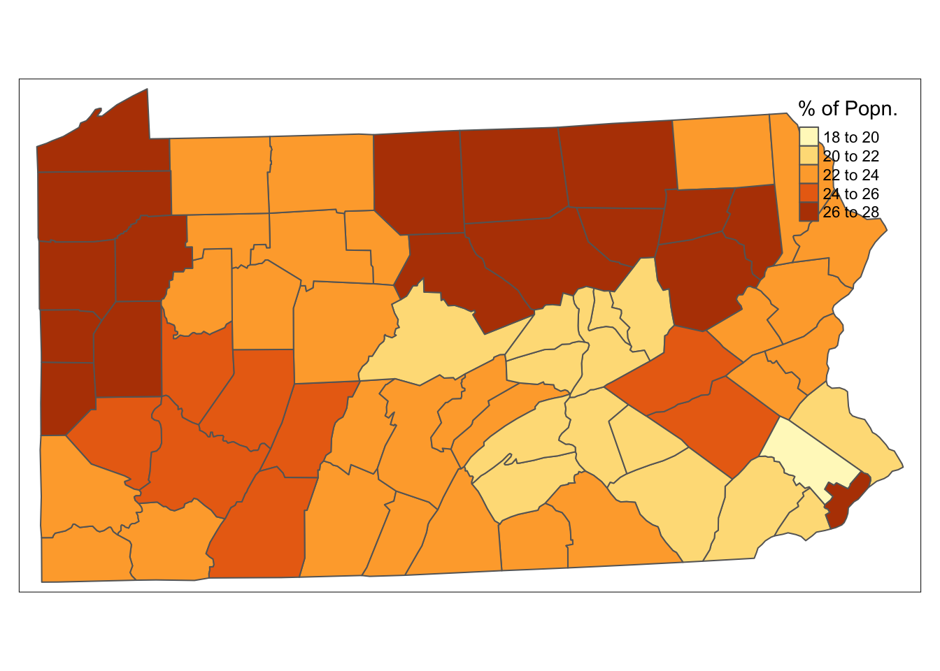
Figure 7.1: Smoking Uptake (Pennysylvania)
7.3 A Visual Exploration of Autocorrelation
# Set up a set of five 'fake' smoking update rates as well as the real one
# Create new columns in penn.state.utm for randomised data
# Here the seed 4676 is used.  Use a different one to get an unknown outcome.

set.seed(4676)
penn.state.utm$smk_rand1 <- sample(penn.state.utm$smk)
penn.state.utm$smk_rand2 <- sample(penn.state.utm$smk)
penn.state.utm$smk_rand3 <- sample(penn.state.utm$smk)
penn.state.utm$smk_rand4 <- sample(penn.state.utm$smk)
penn.state.utm$smk_rand5 <- sample(penn.state.utm$smk)

# Scramble the variables used in terms of plotting order
vars <- sample(c('smk','smk_rand1','smk_rand2','smk_rand3','smk_rand4','smk_rand5'))

# Which one will be the real data?
# Don't look at this variable before you see the maps!
real.data.i <- which(vars == 'smk')

# Draw the scrambled map grid
tm_shape(penn.state.utm) + tm_polygons(col=vars,legend.show=FALSE) +
  tm_layout(title=1:6,title.position=c("right","top"))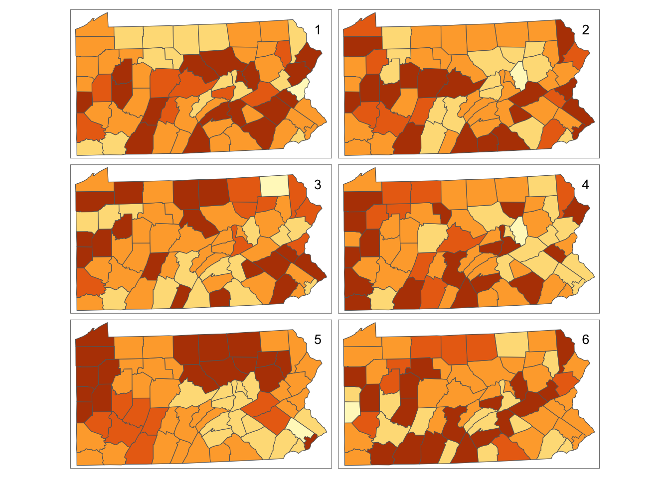
Figure 7.2: Randomisation of smoking uptake rates
[1] 57.3.1 Neighbours and Lagged Mean Plots
Neighbour list object:
Number of regions: 67
Number of nonzero links: 346
Percentage nonzero weights: 7.70773
Average number of links: 5.164179
# Create a SpatialLinesDataFrame showing the Queen's case contiguities
penn.state.net <- nb2lines(penn.state.nb,coords=coordinates(penn.state.utm))
# Default projection is NA, can change this as below
penn.state.net <- set_projection(penn.state.net,current.projection = 3724)
# Draw the projections
tm_shape(penn.state.utm) + tm_borders(col='lightgrey') +
tm_shape(penn.state.net) + tm_lines(col='red')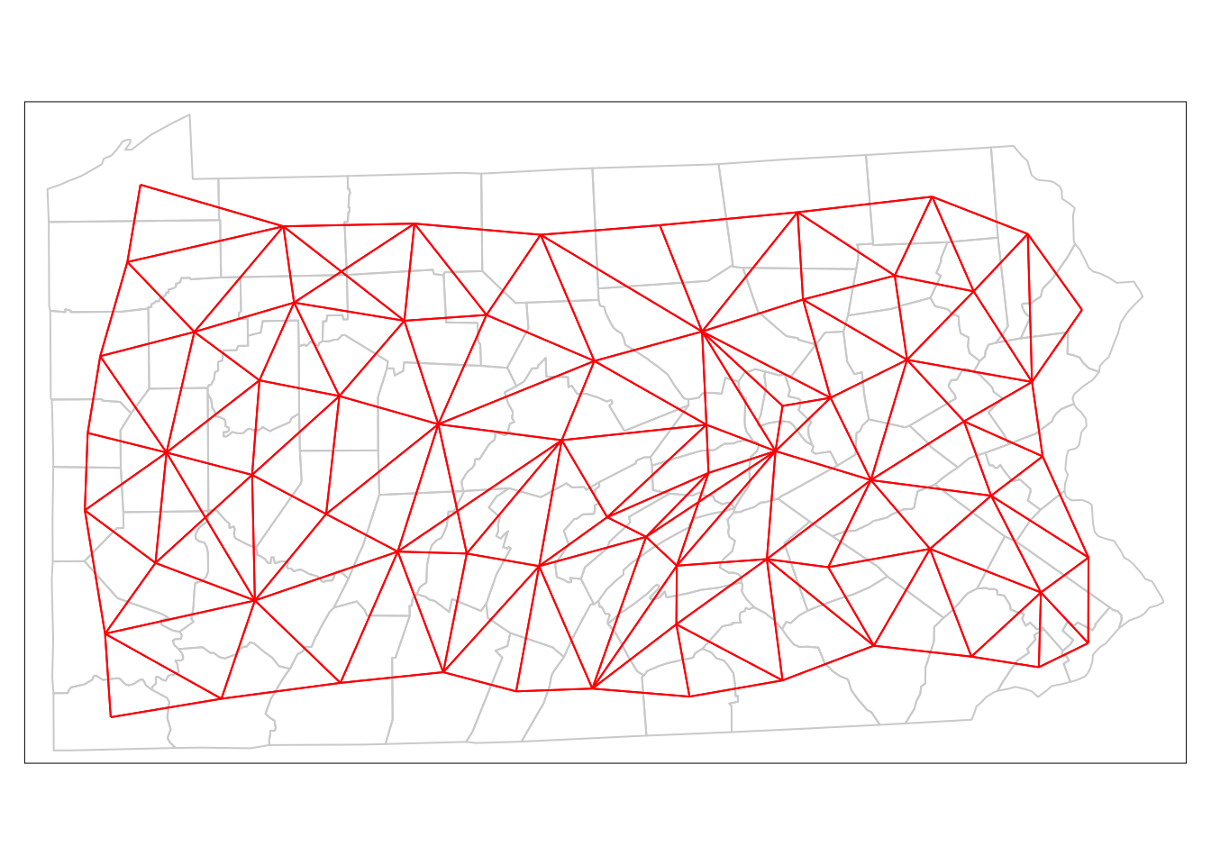
Figure 7.3: Depiction of Neighbouring Counties of Penn State as a network (Queen’s case.)
# Calculate the Rook's case neighbours
penn.state.nb2 <- poly2nb(penn.state.utm,queen=FALSE)
# Convert this to a SpatialLinesDataFrame
penn.state.net2 <- nb2lines(penn.state.nb2,coords=coordinates(penn.state.utm))
# Update prohjection
penn.state.net2 <- set_projection(penn.state.net2,current.projection = 3724)
# Plot the counties in background,  then the two networks to compare:
tm_shape(penn.state.utm) + tm_borders(col='lightgrey') +
  tm_shape(penn.state.net) + tm_lines(col='blue',lwd = 2) +
  tm_shape(penn.state.net2) + tm_lines(col='yellow')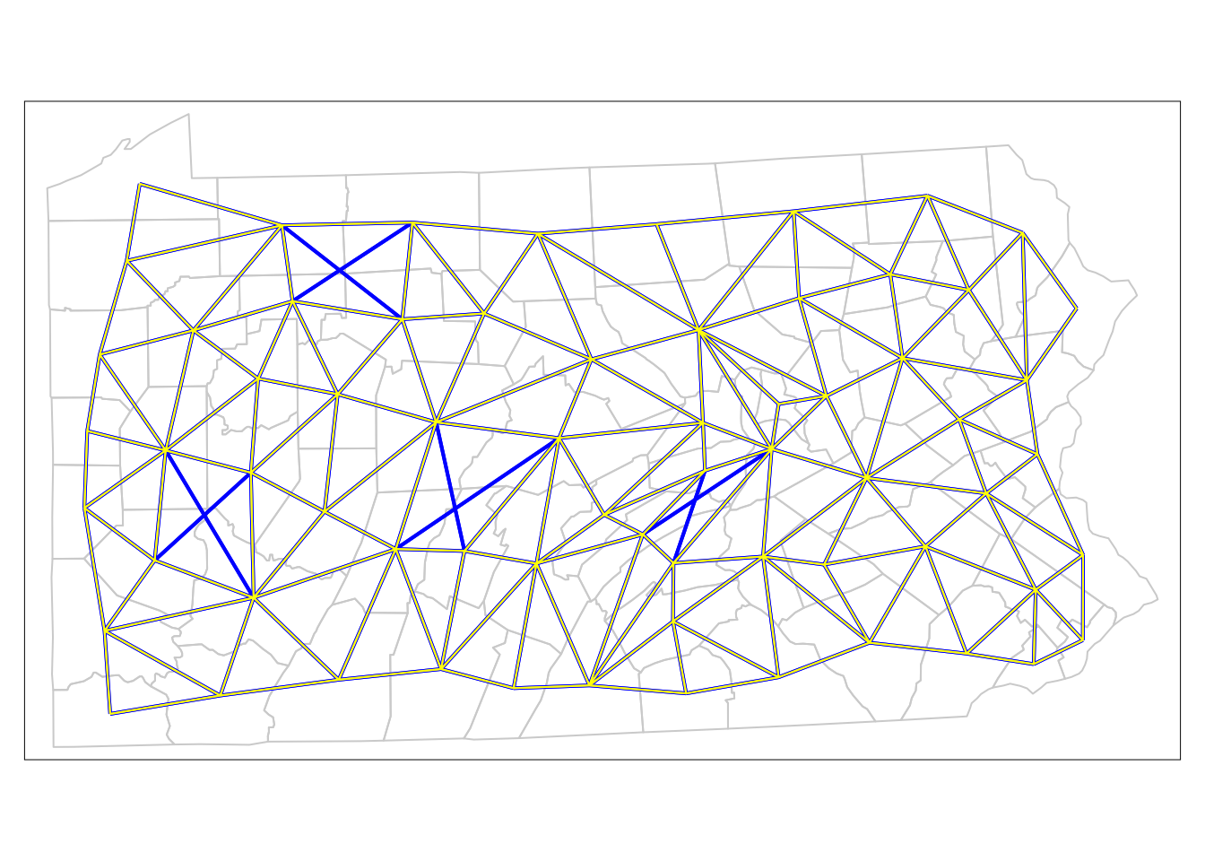
Figure 7.4: Comparison of Neighbouring Counties of Penn State (Rook’s vs. Queen’s case).
# Convert the neighbour list to a listw object - use Rook's case...
penn.state.lw <- nb2listw(penn.state.nb2)
penn.state.lw
Characteristics of weights list object:
Neighbour list object:
Number of regions: 67
Number of nonzero links: 330
Percentage nonzero weights: 7.351303
Average number of links: 4.925373
Weights style: W
Weights constants summary:
n nn S0 S1 S2
W 67 4489 67 28.73789 274.6157penn.state.utm$smk.lagged.means <- lag.listw(penn.state.lw,penn.state.utm$smk)
tm_shape(penn.state.utm) + tm_polygons(col='smk.lagged.means',title='% of Popn.') +
tm_layout(legend.bg.color = "white") 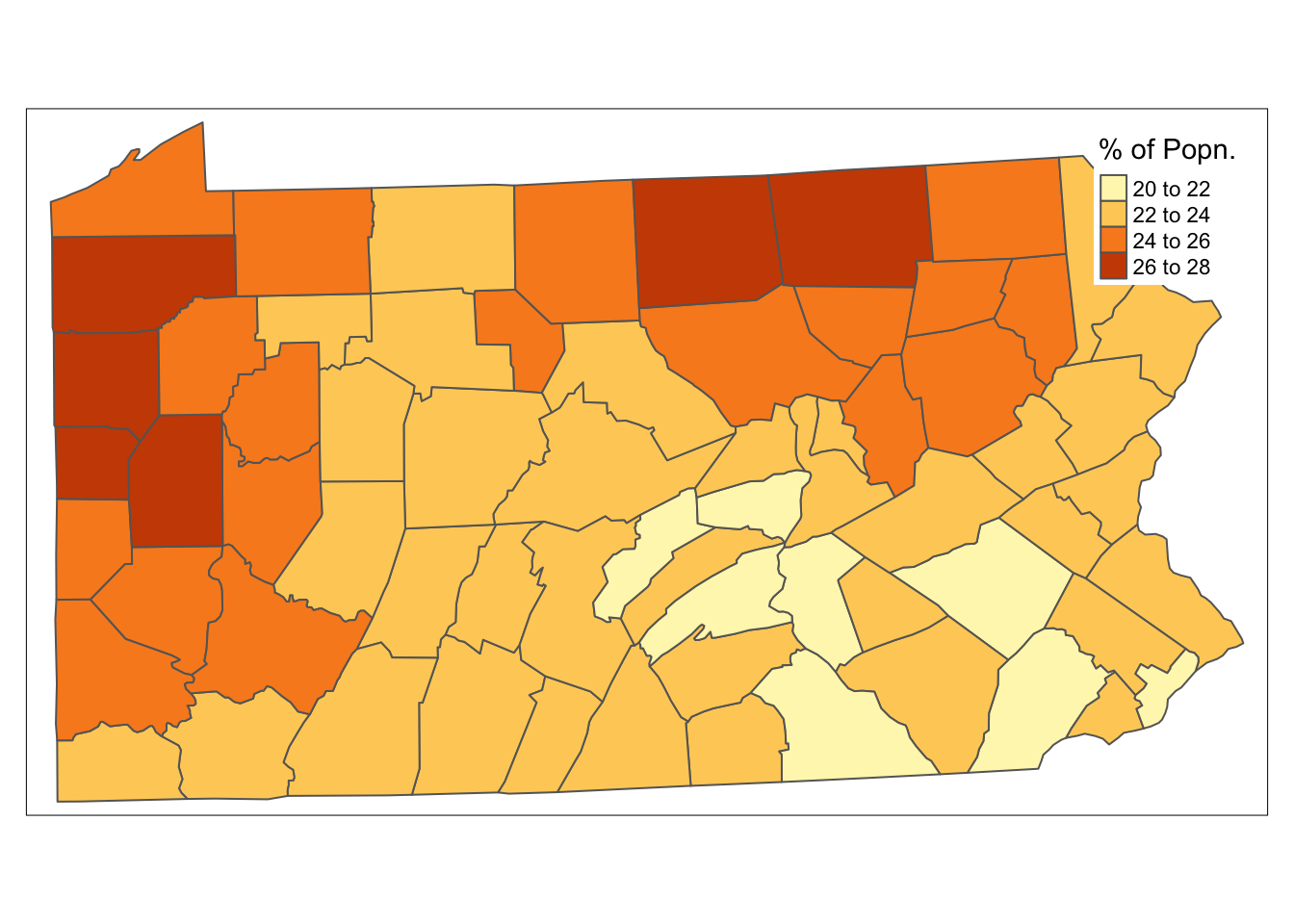
Figure 7.5: Lagged means of smoking uptake rates
with(data.frame(penn.state.utm), {
  plot(smk,smk.lagged.means,asp=1,xlim=range(smk),ylim=range(smk))
  abline(a=0,b=1)
  abline(v=mean(smk),lty=2)
  abline(h=mean(smk.lagged.means),lty=2)
})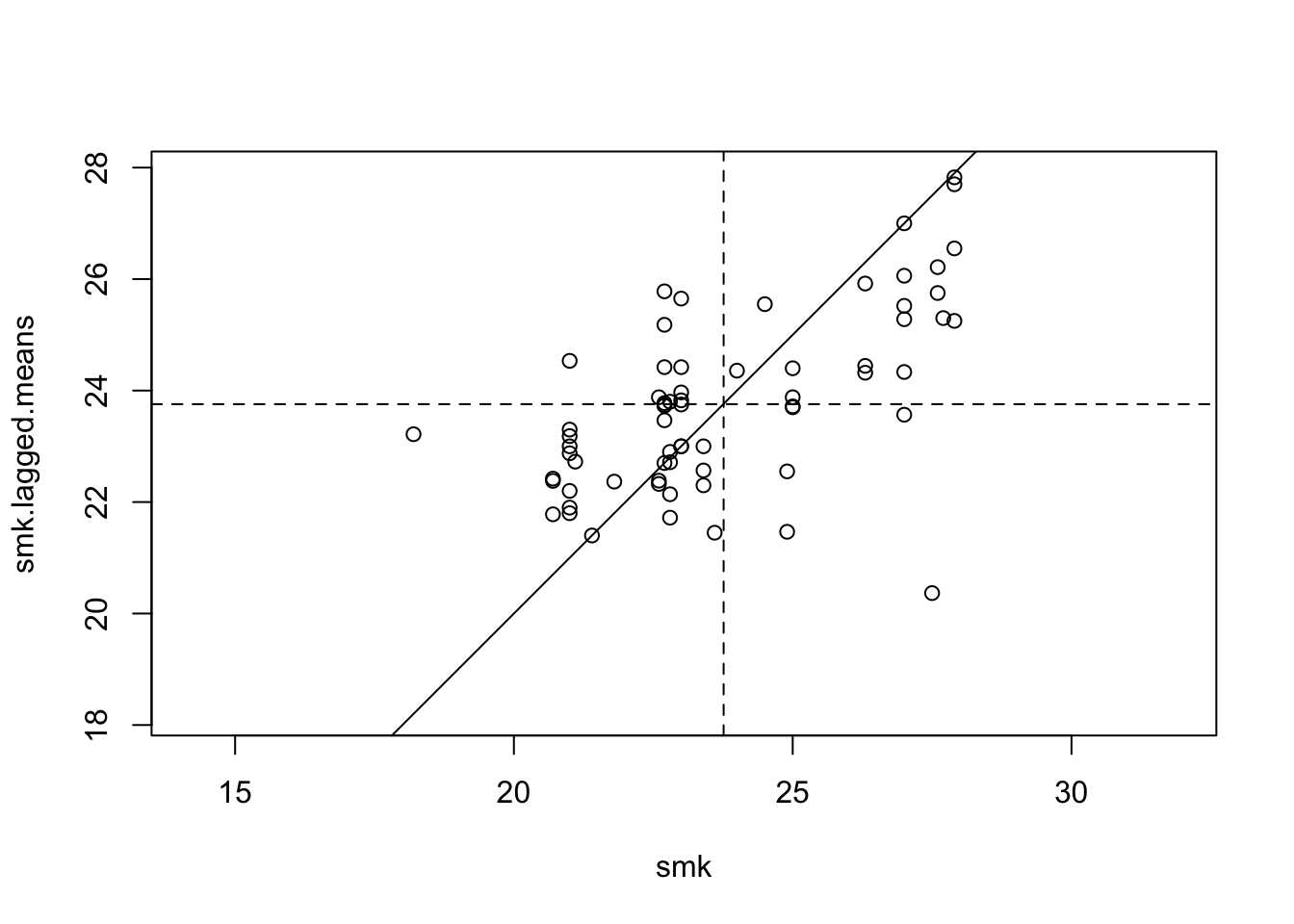
Figure 7.6: Lagged Mean plot for smoking uptake
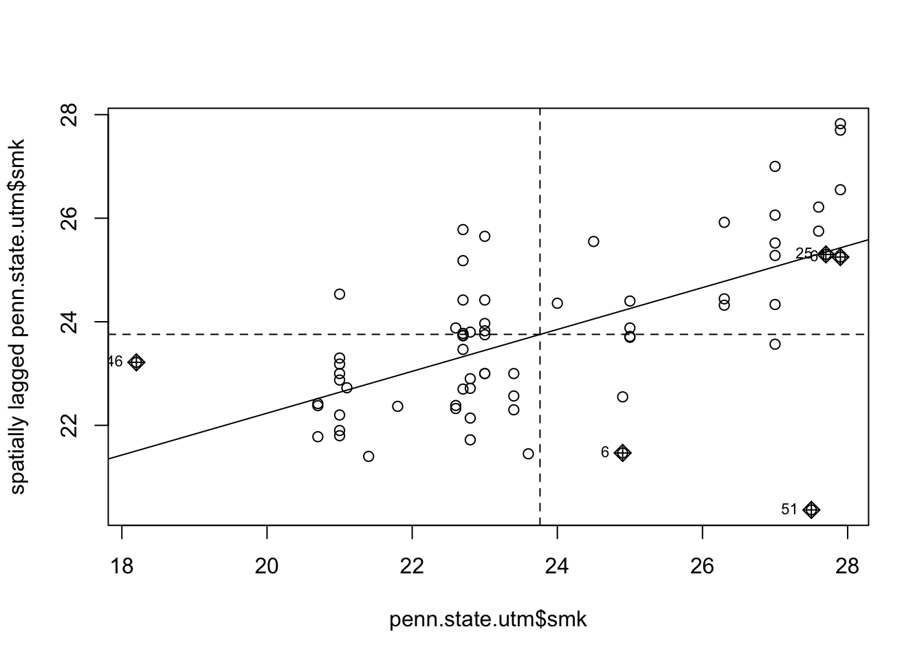
Figure 7.7: Lagged Mean plot for smoking uptake - alternative method.
7.4 Moran’S I: An Index Of Autocorrelation
7.4.1 Moran’s-\(I\) in R
    Moran I test under randomisation

data:  penn.state.utm$smk
weights: penn.state.lw

Moran I statistic standard deviate = 5.4175, p-value
= 3.022e-08
alternative hypothesis: greater
sample estimates:
Moran I statistic       Expectation          Variance
      0.404431265      -0.015151515       0.005998405
moran.range <- function(lw) {
wmat <- listw2mat(lw)
return(range(eigen((wmat + t(wmat))/2)$values))
}
moran.range(penn.state.lw)[1] -0.5785577 1.0202308
    Moran I test under normality

data:  penn.state.utm$smk
weights: penn.state.lw

Moran I statistic standard deviate = 5.4492, p-value
= 2.53e-08
alternative hypothesis: greater
sample estimates:
Moran I statistic       Expectation          Variance
      0.404431265      -0.015151515       0.005928887
7.4.2 A Simulation-Based Approach
    Monte-Carlo simulation of Moran I

data:  penn.state.utm$smk
weights: penn.state.lw
number of simulations + 1: 10001

statistic = 0.40443, observed rank = 10001, p-value =
9.999e-05
alternative hypothesis: greater
note that the third argument provides the number of simulations. Once again, there is evidence to reject the null hypothesis that any permutation of \(z_i\)’s is equally likely in favour of the alternative that \(I > 0\).
7.4.3 Spatial Autoregression
7.5 Calibrating Spatial Regression Models in R
Call:
spautolm(formula = smk ~ 1, data = penn.state.utm, listw = penn.state.lw)

Coefficients:
(Intercept)      lambda
 23.7689073   0.6179367

Log likelihood: -142.8993 [1] 0.1130417[1] 0.3918532 0.84402017.5.1 Models with predictors: A Bivariate Example
  county cases population race gender      age
1  adams     0       1492    o      f Under.40
2  adams     0        365    o      f    40.59
3  adams     1         68    o      f    60.69
4  adams     0         73    o      f      70+
5  adams     0      23351    w      f Under.40
6 adams 5 12136 w f 40.59 county cases population
1 adams 55 91292
2 allegheny 1275 1281666
3 armstrong 49 72392
4 beaver 172 181412
5 bedford 37 49984
6 berks 308 373638 county cases population rate
1 adams 55 91292 6.024624
2 allegheny 1275 1281666 9.947990
3 armstrong 49 72392 6.768704
4 beaver 172 181412 9.481181
5 bedford 37 49984 7.402369
6 berks 308 373638 8.243273# Check the distribution of rates
boxplot(totcases$rate,horizontal=TRUE,
xlab='Cancer Rate (Cases per 10,000 Popn.)')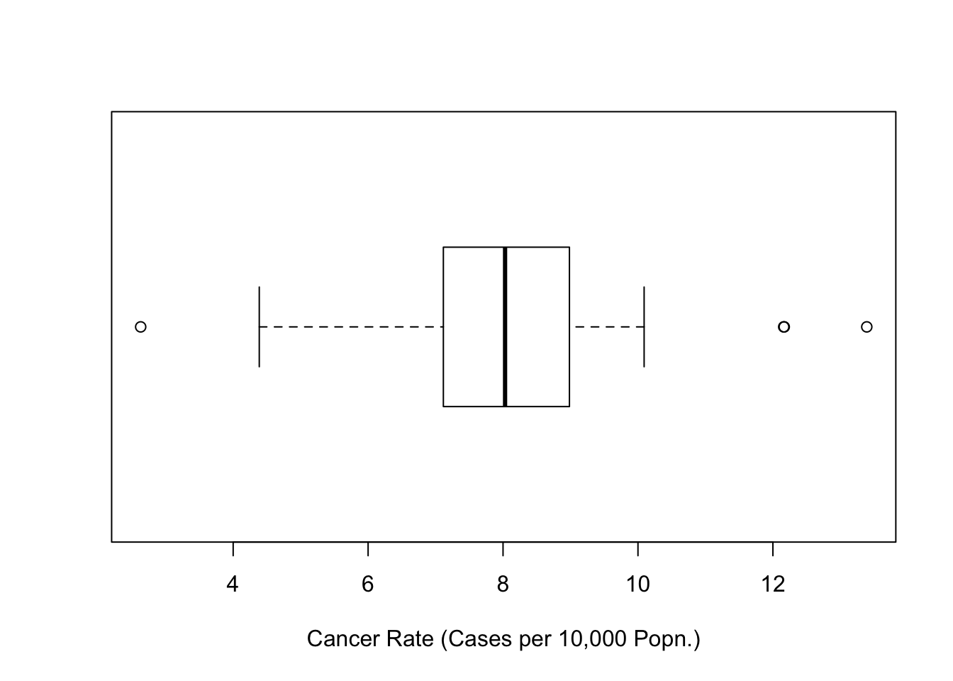
Figure 7.8: Boxplot of Cancer Rates (Penn State 2002)
sar.mod <- spautolm(rate~sqrt(penn.state.utm$smk),listw=penn.state.lw,
                    weight=population,data=totcases)
summary(sar.mod)
Call:
spautolm(formula = rate ~ sqrt(penn.state.utm$smk), data = totcases,
    listw = penn.state.lw, weights = population)

Residuals:
     Min       1Q   Median       3Q      Max
-5.45183 -1.10235 -0.31549  0.59901  5.00115

Coefficients:
                         Estimate Std. Error z value
(Intercept)              -0.35263    2.26795 -0.1555
sqrt(penn.state.utm$smk)  1.80976    0.46064  3.9288
                          Pr(>|z|)
(Intercept)                 0.8764
sqrt(penn.state.utm$smk) 8.537e-05

Lambda: 0.38063 LR test value: 6.3123 p-value: 0.01199
Numerical Hessian standard error of lambda: 0.13984

Log likelihood: -123.3056
ML residual variance (sigma squared): 209030, (sigma: 457.19)
Number of observations: 67
Number of parameters estimated: 4
AIC: 254.61
7.5.2 Further Issues
7.5.3 Troubleshooting Spatial Regression
columbus <- readShapePoly(system.file("etc/shapes/columbus.shp",
 package="spdep")[1])

# Create a plot of columbus and add labels for each of the zones
tm_shape(columbus) + tm_polygons(col='wheat')  +
  tm_text(text='POLYID',size=0.7)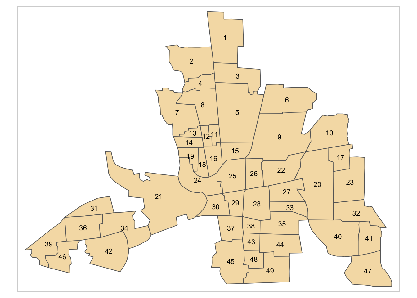
Figure 7.9: Shapefile of neighbourhoods in Columbus, Ohio, with labels
# Extract a 'queen's case' adjacency object and print it out
col.queen.nb <- poly2nb(columbus,queen=TRUE)
col.queen.nb
Neighbour list object:
Number of regions: 49
Number of nonzero links: 236
Percentage nonzero weights: 9.829238
Average number of links: 4.816327 # Extract a 'rooks's case' adjacency object and print it out
col.rook.nb <- poly2nb(columbus,queen=FALSE)
col.rook.nbNeighbour list object:
Number of regions: 49
Number of nonzero links: 200
Percentage nonzero weights: 8.329863
Average number of links: 4.081633 covmat <- function(lambda,adj) {
solve(tcrossprod(diag(length(adj)) - lambda* listw2mat(nb2listw(adj))))
}# Create a range of valid lambda values
lambda.range <- seq(-1.3,0.99,l=101)
# Create an array to store the corresponding correlations
cor.41.47 <- lambda.range*0
# ... store them
for (i in 1:101) cor.41.47[i] <- cormat(lambda.range[i],col.rook.nb)[41,47]
# ... plot the relationship
plot(lambda.range,cor.41.47,type='l')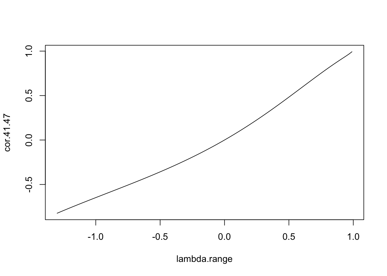
Figure 7.10: Relationship between \(\lambda\) and the correlation between zones 41 and 47
# First, add the line from the previous figure for reference
plot(lambda.range,cor.41.47,type='l',xlab=expression(lambda),ylab='Correlation',lty=2)
# Now compute the correlation between zones 40 and 41.
cor.40.41 <- lambda.range*0
for (i in 1:101) cor.40.41[i] <- cormat(lambda.range[i],col.rook.nb)[40,41]
# ... and add these to the plot
lines(lambda.range,cor.40.41)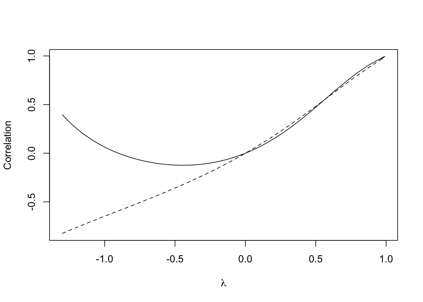
Figure 7.11: Relationship between \(\lambda\) and the correlation between zones 41 and 47
# First,  plot the empty canvas (type='n')
plot(c(-1,1),c(-1,1),type='n',xlim=c(-1,1),ylim=c(-1,1),xlab='Corr1',ylab='Corr2')
# Then the quadrants
rect(-1.2,-1.2,1.2,1.2,col='pink',border=NA)
rect(-1.2,-1.2,0,0,col='lightyellow',border=NA)
rect(0,0,1.2,1.2,col='lightyellow',border=NA)
# Then the x=y reference line
abline(a=0,b=1,lty=3)
# Then the curve
lines(cor.40.41,cor.41.47)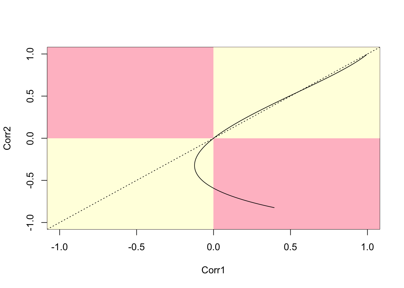
Figure 7.12: Parametric plot of correlations between two polygon pairs (40,41) and (41,47)
# First,  plot the empty canvas (type='n)
plot(c(-1,1),c(-1,1),type='n',xlim=c(-1,1),ylim=c(-1,1),
     xlab='Corr1',ylab='Corr2')
# Then the quadrants
rect(-1.2,-1.2,1.2,1.2,col='pink',border=NA)
rect(-1.2,-1.2,0,0,col='lightyellow',border=NA)
rect(0,0,1.2,1.2,col='lightyellow',border=NA)
# Then the x=y reference line
abline(a=0,b=1,lty=3)
# Then the curves
# First, set a seed for reproducibility
set.seed(310712)
for (i in 1:100) {
  r1 <- sample(1:length(col.rook.nb),1)
  r2 <- sample(col.rook.nb[[r1]],2)
  cor.ij1 <- lambda.range*0
  cor.ij2 <- lambda.range*0
  for (k in 1:101)
    cor.ij1[k] <- cormat(lambda.range[k],col.rook.nb)[r1,r2[1]]
  for (k in 1:101)
    cor.ij2[k] <- cormat(lambda.range[k],col.rook.nb)[r1,r2[2]]
  lines(cor.ij1,cor.ij2)
}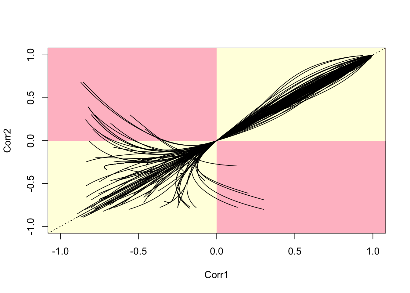
Figure 7.13: Parametric Plots of 100 Sampled Correlations
Answer to self-test question
# Set up a set of five 'fake' smoking update rates as well as the real one
# Create new columns in penn.state.utm for randomised data
# Here the seed 4676 is used.  Use a different one to get an unknown outcome.

set.seed(4676)
penn.state.utm$smk_rand1 <- sample(penn.state.utm$smk,replace=TRUE)
penn.state.utm$smk_rand2 <- sample(penn.state.utm$smk,replace=TRUE)
penn.state.utm$smk_rand3 <- sample(penn.state.utm$smk,replace=TRUE)
penn.state.utm$smk_rand4 <- sample(penn.state.utm$smk,replace=TRUE)
penn.state.utm$smk_rand5 <- sample(penn.state.utm$smk,replace=TRUE)

# Scramble the variables used in terms of plotting order
vars <- sample(c('smk','smk_rand1','smk_rand2','smk_rand3','smk_rand4','smk_rand5'))

# Which one will be the real data?
# Don't look at this variable before you see the maps!
real.data.i <- which(vars == 'smk')

# Draw the scrambled map grid
tm_shape(penn.state.utm) +
  tm_polygons(col=vars,legend.show=FALSE, breaks=c(18,20,22,24,26,28)) +
  tm_layout(title=1:6,title.position=c("right","top"))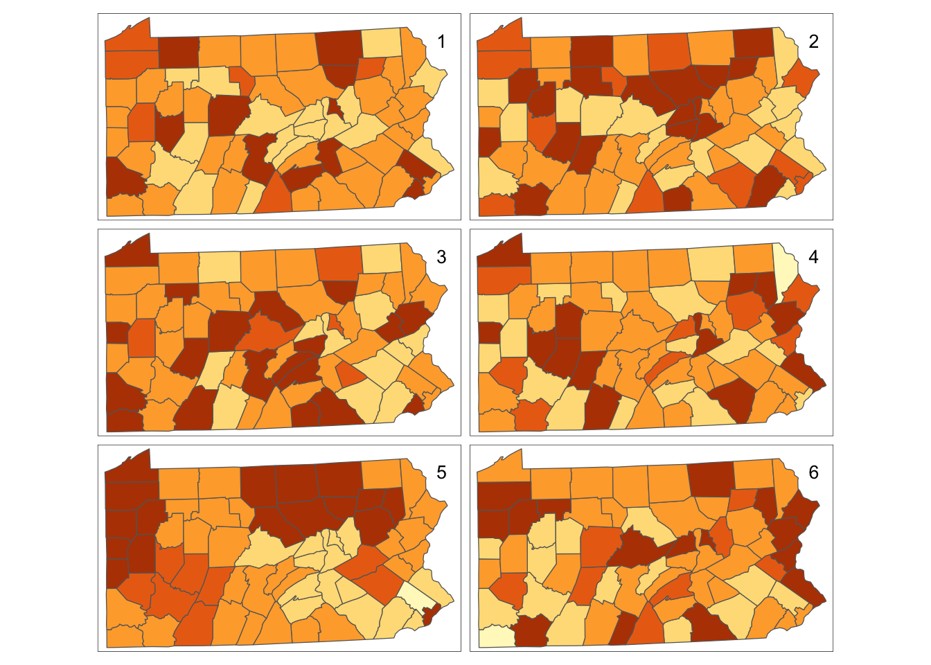
Figure 7.14: Bootstrap Randomisation of smoking uptake rates