Chapter 5 One Sample t-test

Packages used: ggplot2, effectsize.

The first step in a t-test is to look at your data and check your assumptions. We learned how to look at our data in the last chapter (@ref introstat). For this, we are going to switch datasets to the trees dataset. This contains measurements of the diameter in inches (Girth), height in feet (Height), and volume of timber (Volume) of 31 black cherry trees.

#Load up our data
trees <- trees

RQ: Is the average height of trees in the dataset different than 72 feet?

5.1 Get Descriptives

We will use summary() for this, and then run sd() to get the standard deviation.

#Summary statistics
summary(trees$Height)

##    Min. 1st Qu.  Median    Mean 3rd Qu.    Max. 
##      63      72      76      76      80      87

#And the standard deviation
sd(trees$Height)

## [1] 6.371813

5.2 Check Assumptions

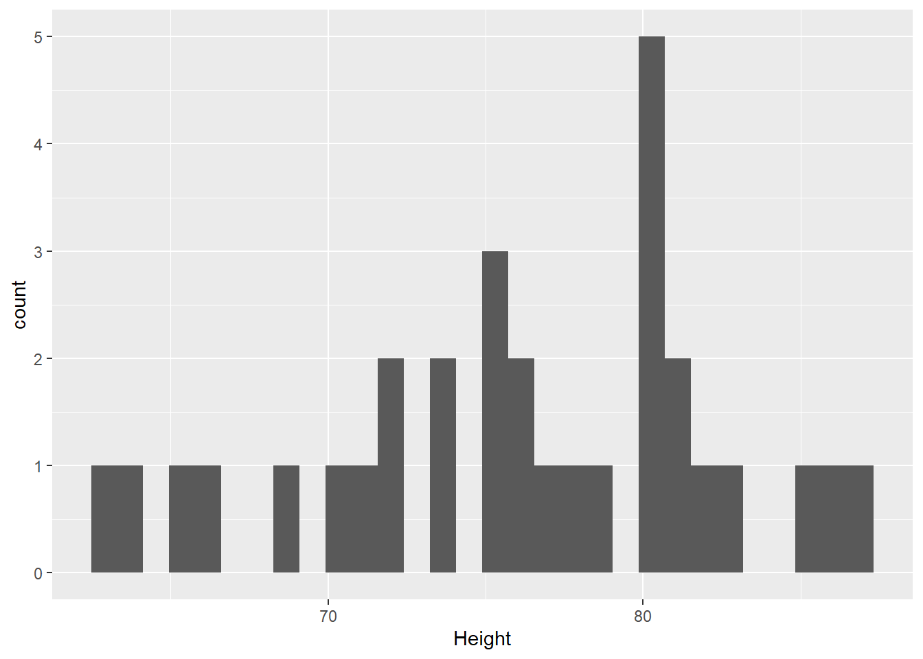
We can see how our data is distributed by using a histogram. ggplot2 is a package with a wide range of graphing capabilities that we will be using for our graphs. There is a later chapter (PUT CHAP REF HERE) specifically on ggplot that explains in more detail what goes with each argument. For this histogram, we are specifying what data to use (trees), and what variable we want to look at (Height). We then say that we would like a histogram (geom_histogram).

#Call ggplot
library(ggplot2)

#Make the plot
ggplot(data = trees, aes(x = Height)) + 
  geom_histogram()

We can see that there may be a slight left skew to the data. To further test this, we can use the Shapiro-Wilk test of normality. Remember that for this test, a non-significant finding indicates that the assumption of normality is satisfied while a significant finding, p < .05, would mean the assumption of normality is violated. The shapiro.test() function in R will be used to test this assumption.

#Shapiro-Wilk test
shapiro.test(trees$Height)

## 
##  Shapiro-Wilk normality test
## 
## data:  trees$Height
## W = 0.96545, p-value = 0.4034

From this output, we see that the p-value = 0.4034. Therefore, these data do not have a distribution that is significantly different than a normal distribution.

5.3 Running the One Sample T-Test: Two-tailed

Recall that we are testing if the average height of the black cherry trees is different than 72 feet. For our one sample t test, 72 is what we will be comparing our mean to, and will be indicated by mu = 72. We will use the t.test() function to run our test, with the following arguments: \[t.test(data, mu = comparison, alternative = "direction")\] where “direction” can take the form “greater” or “less” (we will address this in the next example).

#Run the one sample t test
t.test(trees$Height, mu = 72)

## 
##  One Sample t-test
## 
## data:  trees$Height
## t = 3.4952, df = 30, p-value = 0.001496
## alternative hypothesis: true mean is not equal to 72
## 95 percent confidence interval:
##  73.6628 78.3372
## sample estimates:
## mean of x 
##        76

Looking at the output, we see that it first tells us what data we used: data: trees$Height. The next line is the line we are most interested in. That provides our t-statistic (t = 3.4952), our degrees of freedom (df = 30), and our p-value (p-value = 0.001496). Since the p-value is less than 0.05, we can reject the null hypothesis and conclude that the mean height of black cherry trees in our sample is significantly different than 72.

The output also provides us with a 95% confidence interval. In our case, it is 73.6628, 78.3372.

5.4 Running the One Sample T-Test: One-tailed

We may want to modify our research question to “Is the average height of our black cherry tree sample greater than 72 feet?”. We will use the same function, but add the direction argument (alternative =) to it as below:

#One sample t test, greater
t.test(trees$Height, mu = 72, alternative = "greater")

## 
##  One Sample t-test
## 
## data:  trees$Height
## t = 3.4952, df = 30, p-value = 0.0007478
## alternative hypothesis: true mean is greater than 72
## 95 percent confidence interval:
##  74.05764      Inf
## sample estimates:
## mean of x 
##        76

We see that our output takes the same general format as before, but with different numbers (and a perhaps questionable 95% confidence interval). Our t statistic (t = 3.4952) and degress of freedom (df = 30) remain unchanged. Our p-value (p-value = 0.0007478) has changed, as has our alternative hypothesis (true mean is greater than 72) and 95% confidence interval (74.05764, Inf).

Our conclusion would be slightly different as well: We reject the null hypothesis and conclude that the mean height of our black cherry trees is significantly greater than 72 feet.

5.5 Calculating Cohen’s d

The descriptive statistics we calculated earlier are enough to calculate Cohen’s d by ‘hand’, taking the format \[d = \frac{mean - comparison}{sd}\]. Plugging in our values, we get \[d = \frac{76-72}{6.3718}\]. The math can be done via calculator or within R itself.

#Calculate cohen's d
d <- (76-72)/(6.3718)

#Print the value
d

## [1] 0.6277661

There is also a package that can do this for us, effectsize. The function within that package is cohens_d(), and takes the arguments \[cohens\_d(data, mu = comparison)\].

library(effectsize)

## 
## Attaching package: 'effectsize'

## The following object is masked from 'package:psych':
## 
##     phi

#Get Cohen's d; comparing to a value of 72
cohens_d(trees$Height, mu = 72)

## Cohen's d |       95% CI
## ------------------------
## 0.63      | [0.24, 1.01]
## 
## - Deviation from a difference of 72.

We see that the package-calculated value is the same as our ‘hand’ calculated value: 0.63.