Chapter 14 ANCOVA
Packages used: datarium, psych, tidyverse, ggplot2, viridis, rstatix, broom
The data:
We will be using the “anxiety” data set from the datarium package, which has anxiety score (as a DV), measured at three time points (within-subjects IV) on individuals in three different physical activity groups. The physical activity groups are basal, moderate, and high; in the dataframe they are grp1, grp2, and grp3, respectively. This is the same dataset used in the mixed ANOVA, but we will be modifying it slightly to illustrate ANCOVA procedures. After modifying it, the t1 data point will now be “cov”, or the pre-treatment anxiety level (ie, the covariate), and t3 will be the post anxiety level (ie, treatment effect).
First, we’ll load the data in:
#Call datarium package
library(datarium)

#Assign data set to an object
anx <- anxiety

#See what it looks like
head(anx)
## # A tibble: 6 × 5
## id group t1 t2 t3
## <fct> <fct> <dbl> <dbl> <dbl>
## 1 1 grp1 14.1 14.4 14.1
## 2 2 grp1 14.5 14.6 14.3
## 3 3 grp1 15.7 15.2 14.9
## 4 4 grp1 16 15.5 15.3
## 5 5 grp1 16.5 15.8 15.7
## 6 6 grp1 16.9 16.5 16.2Then, we will modify the data to suit an ANCOVA analysis. We first define a new dataframe, ax, and assign our anx dataframe to it. Then %>% sends the anx dataframe to the next line. select() is saying what columns we want to keep: id, group, t1 and t3. Then, we are renaming these columns for human ease of understanding with rename(). We give the arguments basal = t1, post = t3 to this function to say what the new name is, followed by what the old name was.
After doing all that, we check our work before moving on.
#Load tidyverse for modifications
library(tidyverse)

#Make modifications for an ANCOVA this time
ax <- anx %>%
  select(id, group, t1, t3) %>%
  rename(cov = t1, post = t3)

#Check work
head(ax)
## # A tibble: 6 × 4
## id group cov post
## <fct> <fct> <dbl> <dbl>
## 1 1 grp1 14.1 14.1
## 2 2 grp1 14.5 14.3
## 3 3 grp1 15.7 14.9
## 4 4 grp1 16 15.3
## 5 5 grp1 16.5 15.7
## 6 6 grp1 16.9 16.214.1 Descriptive Statistics
We can look at the means and standard deviations of each group on the pre (cov) and post test anxiety scores.
ax %>%
  group_by(group) %>%
  summarise(mean_cov = mean(cov),
            sd_cov = sd(cov),
            mean_post = mean(post),
            sd_post = sd(post))
## # A tibble: 3 × 5
## group mean_cov sd_cov mean_post sd_post
## <fct> <dbl> <dbl> <dbl> <dbl>
## 1 grp1 17.1 1.63 16.5 1.56
## 2 grp2 16.6 1.57 15.5 1.70
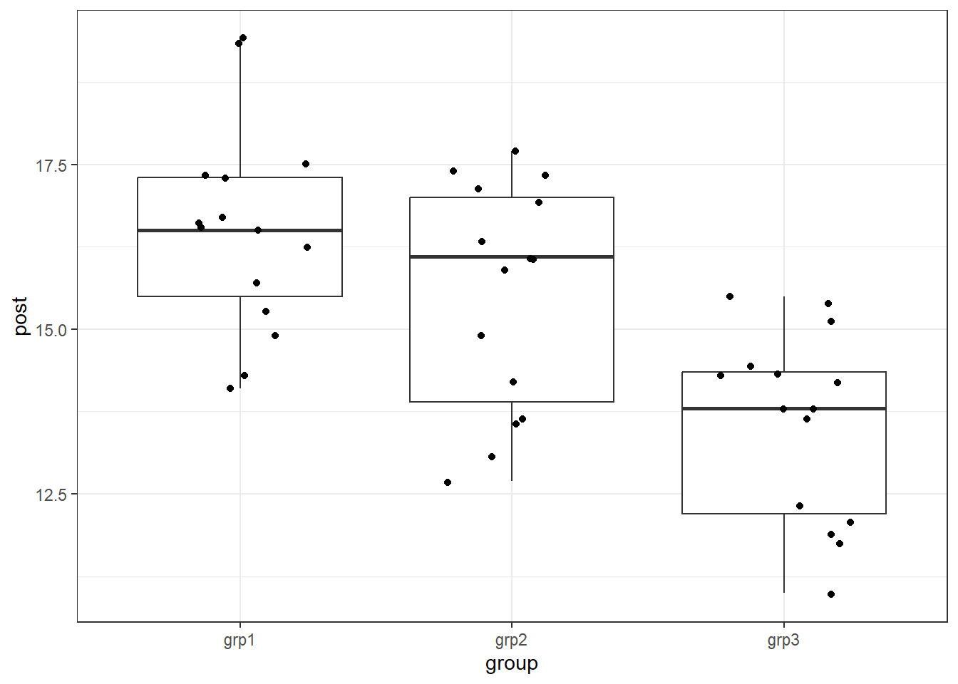
## 3 grp3 17.0 1.32 13.6 1.42We can also examine the distributions of post test scores by group.
#Call ggplot
library(ggplot2)

#Generate a boxplot
ggplot(data = ax, aes(x = group, y = post)) +
  geom_boxplot() +
  geom_jitter(width = .25) +
  theme_bw()
14.2 Assumptions
We will be testing for meeting the assumptions of linearity between the covariate and the outcome variable, homogeneity of regression slopes, normality of residuals, and homogeneity of residuals variance for all groups, and no outliers in the residuals.
14.2.1 Linearity
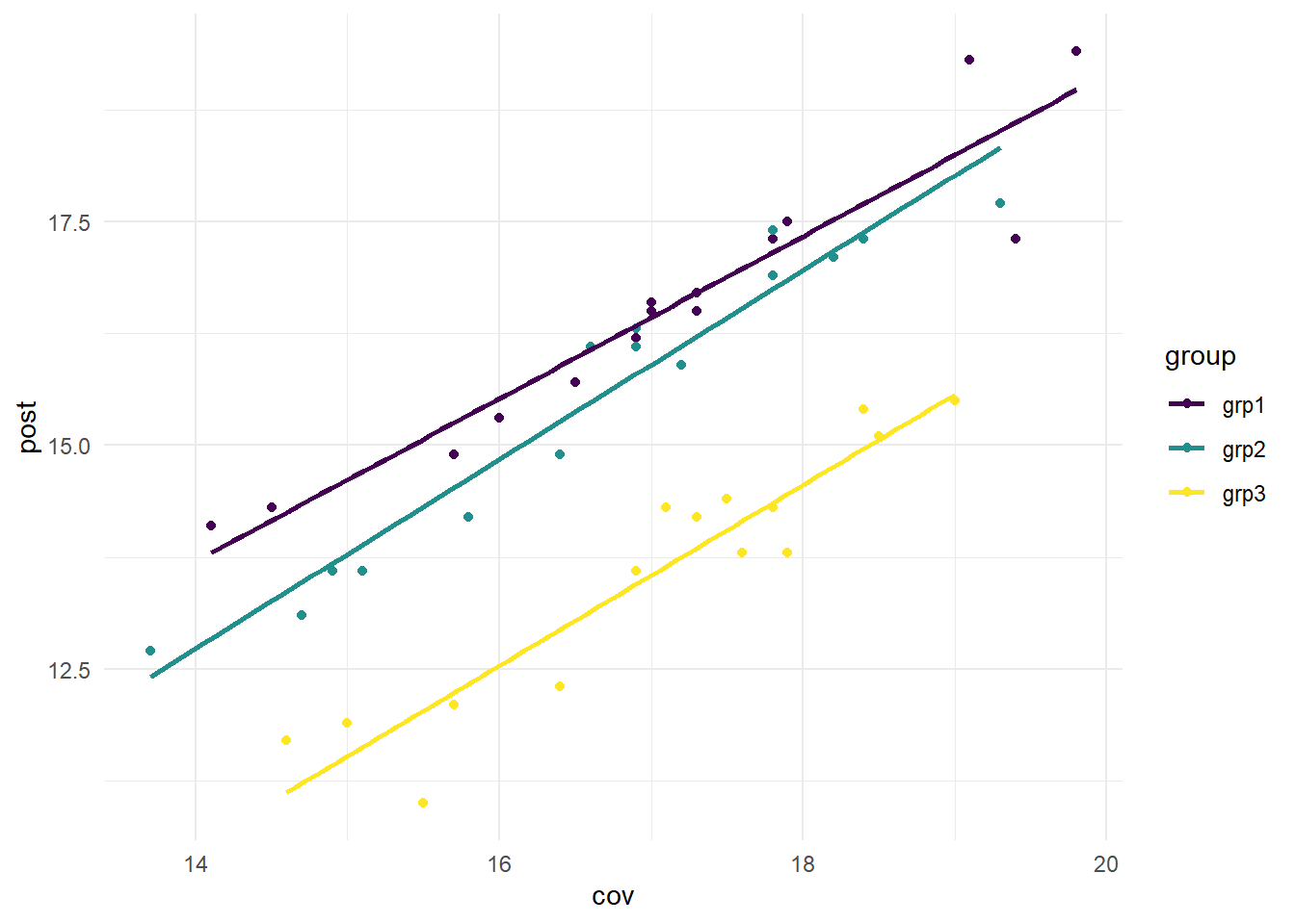
We can test linearity by creating a scatter plot between the covariate (cov; the pre anxiety scores) and the outcome (post; the post anxiety scores). To satisfy this assumption, we are hoping to see a linear relationship between the covariate and outcome for each of our exercise groups.
We will create the scatterplot using ggplot. In the code below, we first call the viridis package, to allow for visual distinction between each of the exercise groups. Then, we have our first call to ggplot: ggplot(data = ax, aes(x = cov, y = post, color = group)) +. This is defining our data (data = ax), the x and y axes (x = cov, y = post), and stating that we want each group to be a different color (color = group). The next line, geom_point() is specifying that we want a scatterplot. To help in determining linear relationships, we add geom_smooth(method = "lm", se = FALSE, aes(color = group)) +. This draws a regression line for each group (method = "lm" specifies a regression line), without standard errors around the line (se = FALSE). The last argument in this line is asking for the regression lines to match the data points (color = group). scale_color_viridis(discrete = TRUE) calls the viridis package, with discrete = TRUE specifying that we are using a discrete, rather than continuous, scale. Lastly, theme_minimal() is addressing the overall background, grid lines, etc.
#Call viridis
library(viridis)

#Make the scatterplot
ggplot(data = ax, aes(x = cov, y = post, color = group)) +
  geom_point() +
  geom_smooth(method = "lm", se = FALSE, aes(color = group)) +
  scale_color_viridis(discrete = TRUE) +
  theme_minimal()
From the graph above, we can see that for each group, there is a linear relationship between the covariate (cov) and the outcome (post). This is a visual inspection, rather than a statistical test.
14.2.2 Homogeneity of Regression Slopes
The homogeneity of regression slopes can be tested by making sure that the interaction between the covariate and the grouping variable (group for us) is not significant. We will test this by running an ANOVA, and checking the interaction term.
In the code below, we are first running an ANOVA using the aov() function, and assigning it to the object assumption_model_ax. Within the aov() function, we first define our formula (post ~ group*cov), followed by our data (data = ax). After running the model, we then ask for an ANOVA table using summary(). This will provide us with the df, SS, MS, F-statistic, and p-value.
#Run the model
assumption_model_ax <- aov(post ~ group*cov, data = ax)

#Get the model summary
summary(assumption_model_ax)
## Df Sum Sq Mean Sq F value Pr(>F)
## group 2 67.56 33.78 145.541 <2e-16 ***
## cov 1 93.37 93.37 402.297 <2e-16 ***
## group:cov 2 0.42 0.21 0.899 0.415
## Residuals 39 9.05 0.23
## ---
## Signif. codes: 0 '***' 0.001 '**' 0.01 '*' 0.05 '.' 0.1 ' ' 1We are only interested in the interaction term in the table above, since we are testing homogeneity of regression slopes. Since it is not significant, we would say this assumption has been met.
14.3 Run the Model to generate residuals
As a difference between ANCOVA and the other ANOVAs we have performed, we need to calculate the model first before we check the assumptions on the residuals (error terms): normality, homoscedasticity, and no outliers.
We will be using lm() to fit the ANCOVA model, as this will allow us to later easily grab the residuals. When we provide the formula to the model, order is important. We want our covariate to go first, followed by the grouping variable. Our model then becomes model_ax <- lm(post ~ cov + group, data = ax). We will next pass our model object to the augment() function from the broom package, which allows us to access the residuals.
#Run the model
model_ax <- lm(post ~ cov + group, data = ax)

#Call the broom package
library(broom)

#Get the residuals
model_ax2 <- augment(model_ax)

#Look at the information provided
head(model_ax2)
## # A tibble: 6 × 9
## post cov group .fitted .resid .hat .sigma .cooksd .std.resid
## <dbl> <dbl> <fct> <dbl> <dbl> <dbl> <dbl> <dbl> <dbl>
## 1 14.1 14.1 grp1 13.6 0.540 0.160 0.478 0.0715 1.23
## 2 14.3 14.5 grp1 14.0 0.346 0.136 0.483 0.0237 0.774
## 3 14.9 15.7 grp1 15.1 -0.238 0.0867 0.485 0.00640 -0.519
## 4 15.3 16 grp1 15.4 -0.134 0.0790 0.486 0.00182 -0.291
## 5 15.7 16.5 grp1 15.9 -0.228 0.0703 0.485 0.00456 -0.492
## 6 16.2 16.9 grp1 16.3 -0.122 0.0670 0.486 0.00125 -0.264Looking at what is contained in the augment() output table, the column we are interested in is the .resid column - those are the residuals on which we need to test the remainder of our assumptions.
14.3.1 Normality
We test the normality of residuals assumption by running a Shapiro-Wilk test with the shapiro.test() function. We specify that we want the Shapriro-Wilk test of the residuals by giving the argument model_ax2$.resid to the function. Pay careful attention to not leave off the “.” from before “resid”. It is a necessary part of the column name.
##
##  Shapiro-Wilk normality test
##
## data:  model_ax2$.resid
## W = 0.96124, p-value = 0.1362