| (x, y) | P(X = x, Y = y) |
|---|---|
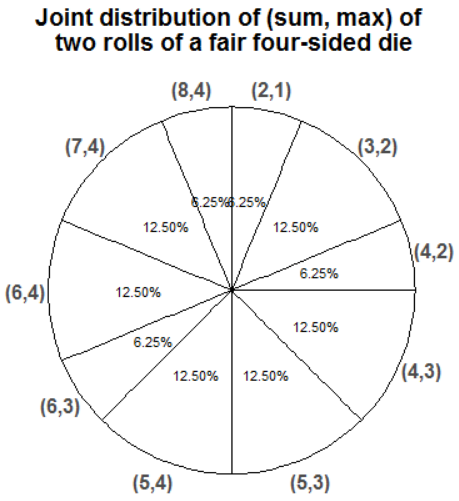
| (2, 1) | 0.0625 |
| (3, 2) | 0.1250 |
| (4, 2) | 0.0625 |
| (4, 3) | 0.1250 |
| (5, 3) | 0.1250 |
| (5, 4) | 0.1250 |
| (6, 3) | 0.0625 |
| (6, 4) | 0.1250 |
| (7, 4) | 0.1250 |
| (8, 4) | 0.0625 |
12 Joint Distributions
Example 12.1 Roll a fair four-sided die twice. Let \(X\) be the sum of the two dice, and let \(Y\) be the larger of the two rolls (or the common value if both rolls are the same). Recall Table 5.1.
- Compute and interpret \(p_{X, Y}(5, 3) = \text{P}(X = 5, Y = 3)\).
- Construct a “flat” table displaying the distribution of \((X, Y)\) pairs, with one pair in each row.
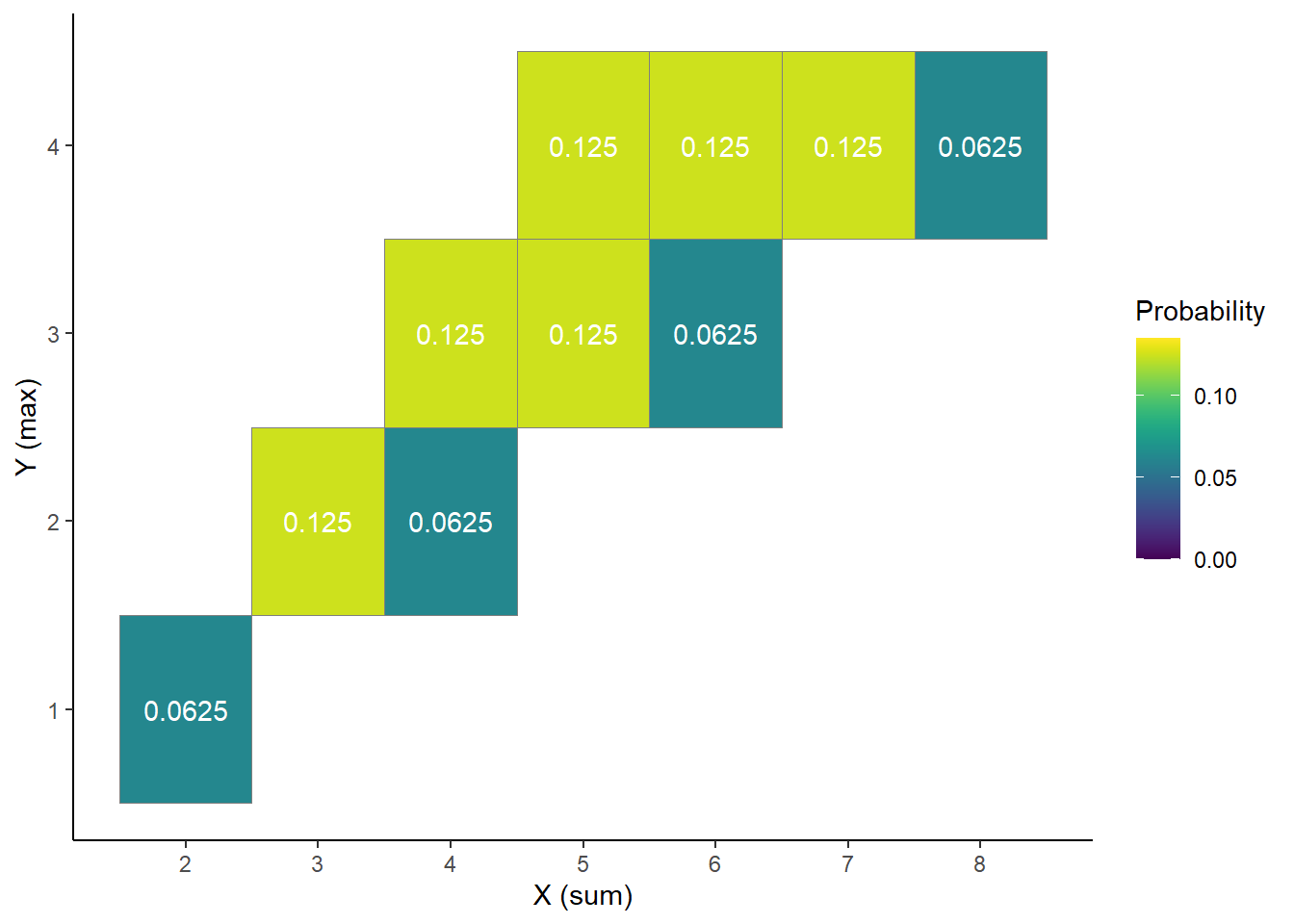
- Construct a two-way displaying the joint distribution on \(X\) and \(Y\).
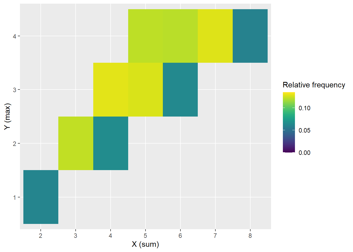
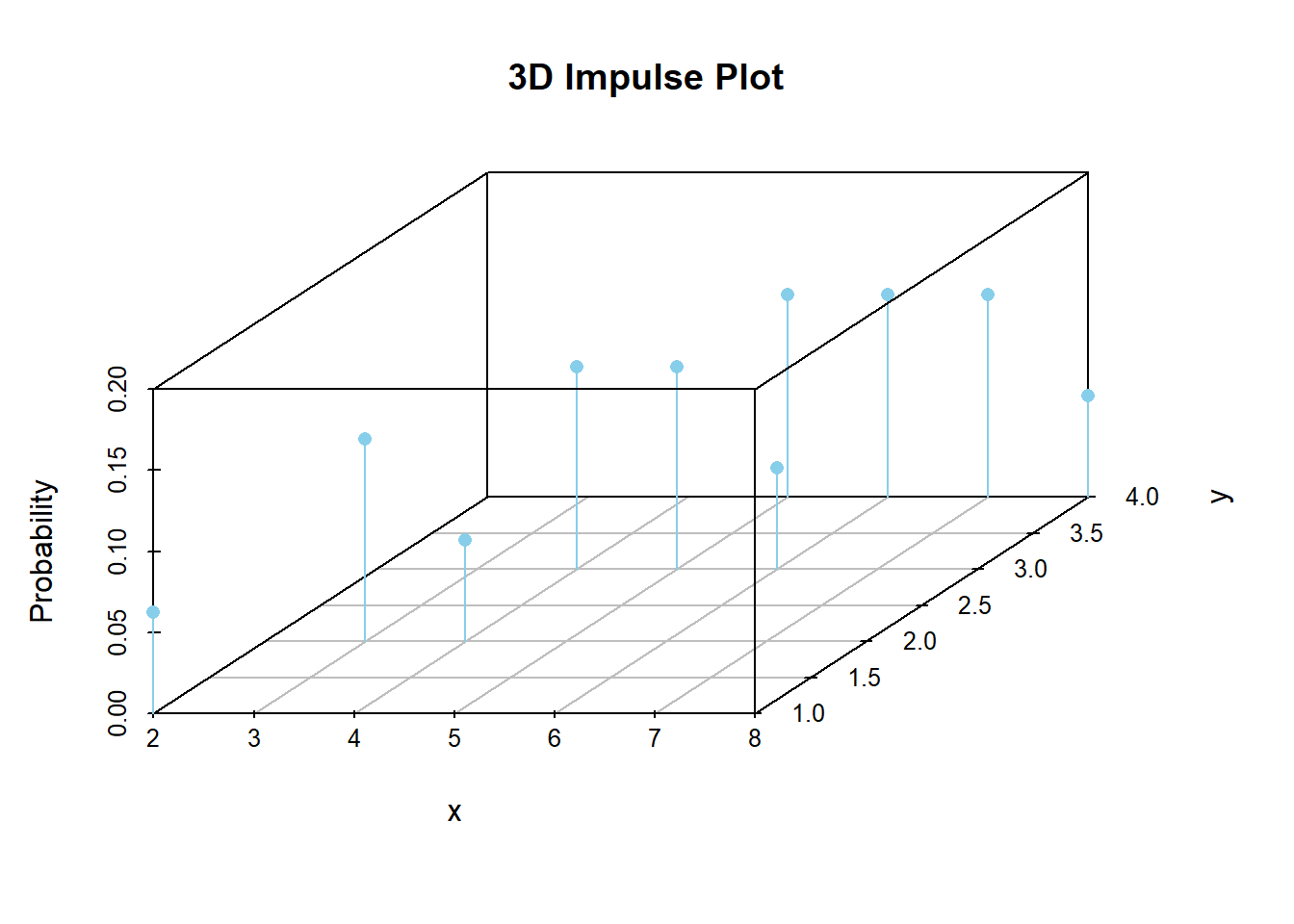
- Sketch a plot depicting the joint distribution of \(X\) and \(Y\).
- Starting with the two-way table, how could you obtain \(\text{P}(X = 5)\)?
- Starting with the two-way table, how could you obtain the marginal distribution of \(X\)? of \(Y\)?
- Starting with the marginal distribution of \(X\) and the marginal distribution of \(Y\), could you necessarily construct the two-way table of the joint distribution? Explain.
- The joint distribution of random variables \(X\) and \(Y\) is a probability distribution on \((x, y)\) pairs, and describes how the values of \(X\) and \(Y\) vary together or jointly.
- Marginal distributions can be obtained from a joint distribution by “stacking”/“collapsing”/“aggregating” out the other variable.
- In general, marginal distributions alone are not enough to determine a joint distribution. (The exception is when random variables are independent.)
| \(x\) \ \(y\) | 1 | 2 | 3 | 4 |
| 2 | 1/16 | 0 | 0 | 0 |
| 3 | 0 | 2/16 | 0 | 0 |
| 4 | 0 | 1/16 | 2/16 | 0 |
| 5 | 0 | 0 | 2/16 | 2/16 |
| 6 | 0 | 0 | 1/16 | 2/16 |
| 7 | 0 | 0 | 0 | 2/16 |
| 8 | 0 | 0 | 0 | 1/16 |
Example 12.2 Continuing the dice rolling example, construct a spinner representing the joint distribution of \(X\) and \(Y\).
N_rep = 16000

# first roll
u1 = sample(1:4, size = N_rep, replace = TRUE)

# second roll
u2 = sample(1:4, size = N_rep, replace = TRUE)

# sum
x = u1 + u2

# max
y = pmax(u1, u2)

dice_sim = data.frame(u1, u2, x, y)| Repetition | First roll | Second roll | X (sum) | Y (max) |
|---|---|---|---|---|
| 1 | 2 | 1 | 3 | 2 |
| 2 | 1 | 2 | 3 | 2 |
| 3 | 1 | 3 | 4 | 3 |
| 4 | 4 | 2 | 6 | 4 |
| 5 | 2 | 3 | 5 | 3 |
| 6 | 2 | 3 | 5 | 3 |
# Joint distribution: counts
table(x, y)
y
x 1 2 3 4
2 980 0 0 0
3 0 1960 0 0
4 0 1039 2070 0
5 0 0 2038 1948
6 0 0 1017 1935
7 0 0 0 2052
8 0 0 0 961# Joint distribution: proportions
table(x, y) / N_rep y
x 1 2 3 4
2 0.0612500 0.0000000 0.0000000 0.0000000
3 0.0000000 0.1225000 0.0000000 0.0000000
4 0.0000000 0.0649375 0.1293750 0.0000000
5 0.0000000 0.0000000 0.1273750 0.1217500
6 0.0000000 0.0000000 0.0635625 0.1209375
7 0.0000000 0.0000000 0.0000000 0.1282500
8 0.0000000 0.0000000 0.0000000 0.0600625sum((x == 5) * (y == 3)) / N_rep[1] 0.127375library(tidyverse)
library(viridis)
ggplot(dice_sim |>
# changing to factor ("categorical" helps with plotting)
mutate(x = factor(x), y = factor(y)),
aes(x = x, y = y)) +
# fill color is relative frequency
stat_bin_2d(aes(fill = after_stat(count) / sum(after_stat(count)))) +
# color scale
scale_fill_viridis(limits = c(0, 2 / 16 + 0.01)) +
# labels
labs(x = "X (sum)",
y = "Y (max)",
fill = "Relative frequency")