7  Expected Value

• The distribution of a random variable specifies the possible values and the probability of any event that involves the random variable.
• The distribution of a random variable contains all the information about its long run behavior. It is also useful to summarize some key features of a distribution.
• One summary characteristic of a distribution is the long run average value of the random variable.
• We can approximate the long run average value by simulating many values of the random variable and computing the average (mean) in the usual way: sum the simulated values and divide by the number of simulated values.

Example 7.1 Recall the matching problem with $n=4$. Table 7.1 displays the value of $X$, the number of matches, for 10 simulated repetitions.

Table 7.1: The value of $X$, the number of matches, for 10 simulated repetitions of the matching problem with $n=4$.

Repetition	X (number of matches)
1	0
2	1
3	0
4	0
5	2
6	0
7	1
8	1
9	4
10	2

1. How could you use the simulation results to approximate the long run average value of $X$? How could you get a better approximation of the long run average?
   
   
   
   
   
2. Rather than adding the 10 values and dividing by 10, how could you simplify the calculation in the previous part?
   
   
   
   
   
3. Table 7.2 below summarizes 24000 simulated values of $X$. Approximate the long run average value of $X$.
   
   
   
   
   
4. Recall the distribution of $X$ from Example 5.4. What would be the corresponding mathematical formula for the theoretical long run average value of $X$? This number is called the “expected value” of $X$.
   
   
   
   
   
5. Is the expected value the most likely value of $X$?
   
   
   
   
   
6. Is the expected value of $X$ the “value that we would expect” on a single repetition of the matching problem?
   
   
   
   
   
7. Explain in what sense the expected value is “expected”.
   
   
   
   
   

# One repetition of the number of matches, for a given n
simulate_number_matches = function(n) {
  # sample(1:n) puts the values 1:n in random order
  sum(sample(1:n) == 1:n)
}

# Many repetitions, for n = 4
N_rep = 24000
number_matches = replicate(N_rep, simulate_number_matches(4))

# Summarize the simulated values
table(number_matches) |>
  as.data.frame() |>
  adorn_totals("row") |>
  kbl(col.names = c("Number of Matches (X)",
                    "Frequency")) |>
  kable_styling(fixed_thead = TRUE)

Table 7.2: Summary of 24000 simulated values of $X$, the number of matches, in the matching problem with $n=4$.

Number of Matches (X)	Frequency
0	8953
1	8102
2	5908
4	1037
Total	24000

sum(number_matches)

[1] 24066

sum(number_matches) / N_rep

[1] 1.00275

mean(number_matches)

[1] 1.00275

• The expected value (a.k.a. expectation a.k.a. mean), of a random variable $X$ is a number denoted $\text{E}(X)$ representing the probability-weighted average value of $X$.
• The expected value of a discrete random variable with pmf $p_X$ is defined as $$\text{E}(X)=\sum _{x}x{p}_X(x)=\sum \text{value}\times \text{probability}$$
• Note well that $\text{E}(X)$ represents a single number.
• The expected value is the “balance point” (center of gravity) of a distribution.
• The expected value of a random variable $X$ is defined by the probability-weighted average according to the underlying probability measure. But the expected value can also be interpreted as the long-run average value, and so can be approximated via simulation.
• Read the symbol $\text{E}(\cdot )$ as
  • Simulate lots of values of what’s inside $(\cdot )$
  • Compute the average. This is a “usual” average; just sum all the simulated values and divide by the number of simulated values.

Table 7.3: Running average of 10 simulated values of $X$ in the matching problem with $n=4$.

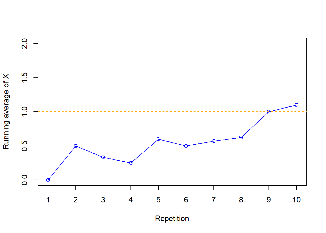
Repetition	Value of X	Running average of X
1	0	0.000
2	1	0.500
3	0	0.333
4	0	0.250
5	2	0.600
6	0	0.500
7	1	0.571
8	1	0.625
9	4	1.000
10	2	1.100

Figure 7.1: Running average of 10 simulated values of $X$ in the matching problem with $n=4$.

Figure 7.2: Running average of 100 simulated values of $X$ in the matching problem with $n=4$.

Figure 7.3: Running average of 1000 simulated values of $X$ in the matching problem with $n=4$.

Example 7.2 Continuing Example 6.2. Consider an extremely simplified model for the daily closing price of a certain stock. Every day the price either goes up or goes down, and the movements are independent from day-to-day. Assume that the probability that the stock price goes up on any single day is 0.25. Let $X$ be the number of days in which the price goes up in the next 5 days.

1. Suggest a shortcut formula for $\text{E}(X)$.
   
   
   
   
   
2. Compute $\text{E}(X)$ using the distribution of $X$ from Example 6.2. Did the shortcut formula work?
   
   
   
   
   
3. Interpret $\text{E}(X)$.
   
   
   
   
   

• If $X$ has a Binomial($n$, $p$) distribution then $\text{E}(X)=np$.

Example 7.3 Continuing Example 6.1. Assume that $X$, the number of home runs hit (in total by both teams) in a randomly selected Major League Baseball game, follows a Poisson(2.3) distribution.

1. Compute $\text{E}(X)$.
   
   
   
   
   
   
2. Interpret $\text{E}(X)$ in context.
   
   
   
   
   

• If $X$ has a Poisson($\mu$) distribution then $\text{E}(X)=\mu$.