N_rep = 16000

# first roll
u1 = sample(1:4, size = N_rep, replace = TRUE)

# second roll
u2 = sample(1:4, size = N_rep, replace = TRUE)

# sum
x = u1 + u2

# max
y = pmax(u1, u2)13 Covariance and Correlation
Quantities like expected value and variance summarize characteristics of the marginal distribution of a single random variable. When there are multiple random variables their joint distribution is of interest. Covariance and correlation summarize a characteristic of the joint distribution of two random variables, namely, the degree to which they “co-deviate from the their respective means”.
13.1 Covariance
- The covariance between two random variables \(X\) and \(Y\) is \[\begin{align*} \text{Cov}(X,Y) & = \text{E}\left[\left(X-\text{E}[X]\right)\left(Y-\text{E}[Y]\right)\right]\\ & = \text{E}(XY) - \text{E}(X)\text{E}(Y) \end{align*}\]
- Covariance is the long run average of the products of the paired deviations from the mean
- Covariance is the expected value of the product minus the product of expected values.
Example 13.1 Roll a fair four-sided die twice and let \(X\) be the sum of the two rolls, and \(Y\) the larger of the two rolls.
- Specify the joint pmf of \(X\) and \(Y\). (These first few parts are review of things we have covered before.)
- Find the marginal pmf of \(X\) and \(\text{E}(X)\).
- Find the marginal pmf of \(Y\) and \(\text{E}(Y)\).
- Find \(\text{E}(XY)\). Is it equal to \(\text{E}(X)\text{E}(Y)\)?
- Find \(\text{Cov}(X, Y)\). Why is the covariance positive?
- Describe how you would use simulation to approximate \(\text{Cov}(X, Y)\).
| Repetition | X | Y | XY | X - E(X) | Y - E(Y) | (X-E(X))(Y-E(Y)) |
|---|---|---|---|---|---|---|
| 1 | 6 | 3 | 18 | 1 | -0.125 | -0.125 |
| 2 | 8 | 4 | 32 | 3 | 0.875 | 2.625 |
| 3 | 5 | 4 | 20 | 0 | 0.875 | 0.000 |
| 4 | 4 | 2 | 8 | -1 | -1.125 | 1.125 |
| 5 | 6 | 4 | 24 | 1 | 0.875 | 0.875 |
| 6 | 7 | 4 | 28 | 2 | 0.875 | 1.750 |
mean((x - mean(x)) * (y - mean(y)))[1] 1.238242mean(x * y)[1] 16.80006mean(x * y) - mean(x) * mean(y)[1] 1.238242cov(x, y)[1] 1.238319- \(\text{Cov}(X,Y)>0\) (positive association): above average values of \(X\) tend to be associated with above average values of \(Y\)
- \(\text{Cov}(X,Y)<0\) (negative association): above average values of \(X\) tend to be associated with below average values of \(Y\)
- \(\text{Cov}(X,Y)=0\) indicates that the random variables are uncorrelated: there is no overall positive or negative association. But be careful: if \(X\) and \(Y\) are uncorrelated there can still be a relationship between \(X\) and \(Y\); there is just no overall positive or negative association.. We will see examples that demonstrate that being uncorrelated does not necessarily imply that random variables are independent.
Example 13.2 Continuing Example 13.1. Let \(X\) be the sum of the two rolls, \(Y\) the larger of the two rolls, \(W\) the number of rolls equal to 4, and \(Z\) the number of rolls equal to 1.
- Is \(\text{Cov}(X, W)\) positive, negative, or zero? Why?
- Is \(\text{Cov}(X, Z)\) positive, negative, or zero? Why?
- Let \(V=W+Z\). Is \(\text{Cov}(X, V)\) positive, negative, or zero? Why?
- Is \(\text{Cov}(W, Z)\) positive, negative, or zero? Why?
# 4s
w = (u1 == 4) + (u2 == 4)

# 1s
z = (u1 == 1) + (u2 == 1)

# 4s or 1s
v = w + z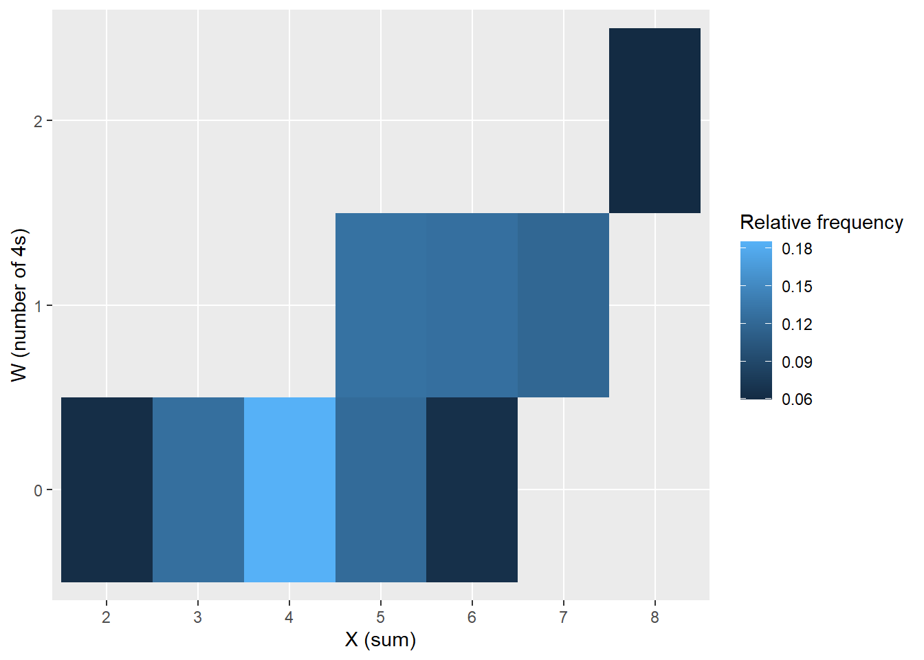
cov(x, w)[1] 0.7332768cor(x, w)[1] 0.7679727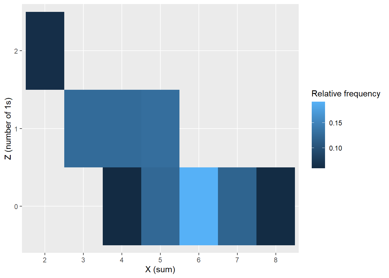
cov(x, z)[1] -0.7490746cor(x, z)[1] -0.7777664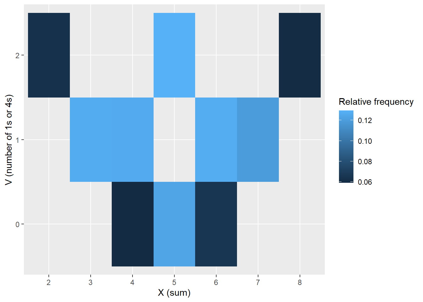
cov(x, v)[1] -0.01579782cor(x, v)[1] -0.01422041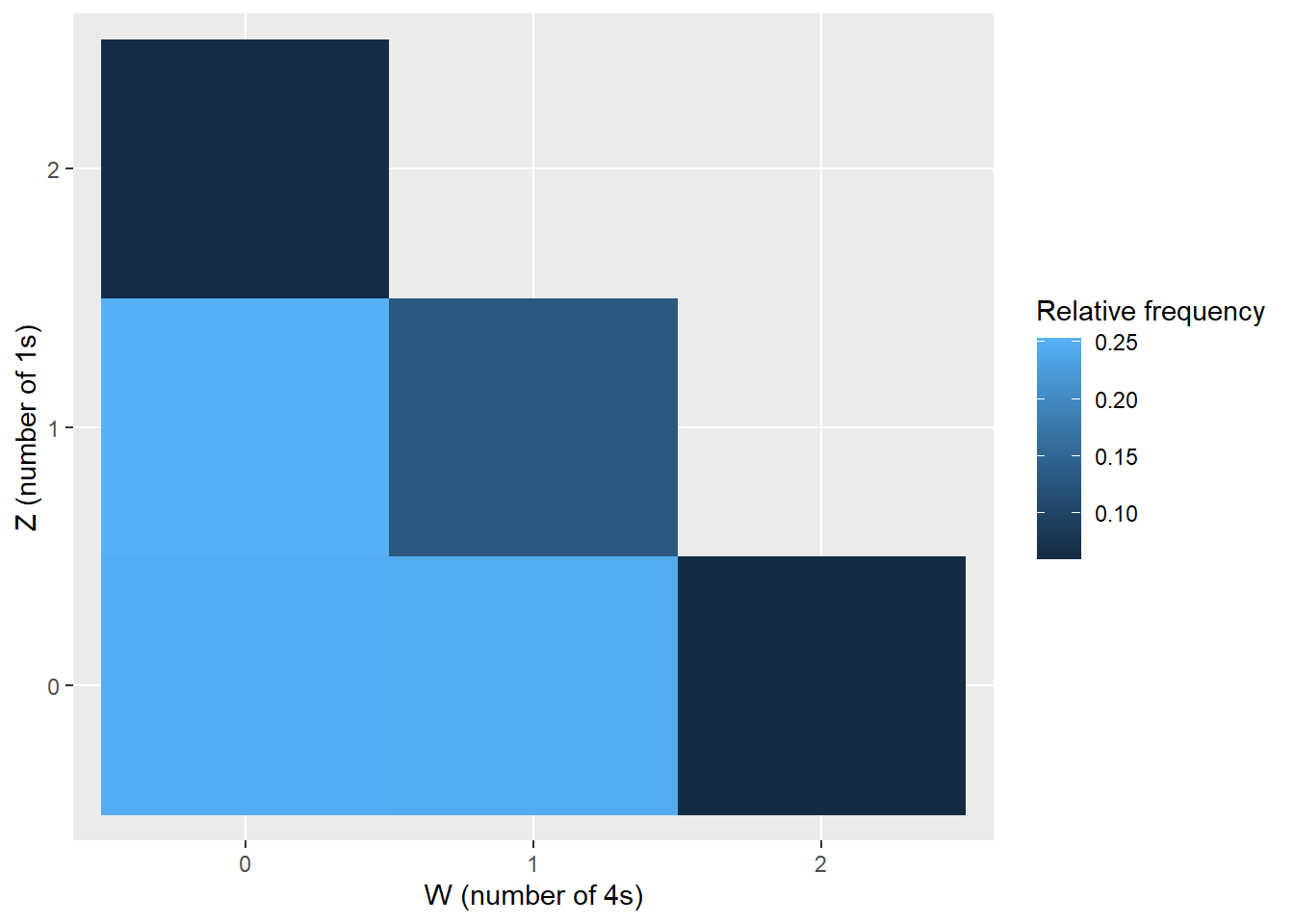
cov(w, z)[1] -0.1226243cor(w, z)[1] -0.3290068Example 13.3 What is another name for \(\text{Cov}(X, X)\)?
13.2 Correlation
Example 13.4 The covariance between height in inches and weight in pounds for football players is 96.
- What are the measurement units of the covariance?
- Suppose height were measured in feet instead of inches. Would the shape of the joint distribution change? Would the strength of the association between height and weight change? Would the value of covariance change?
- The correlation (coefficient) between random variables \(X\) and \(Y\) is \[\begin{align*} \text{Corr}(X,Y) & = \text{Cov}\left(\frac{X-\text{E}(X)}{\text{SD}(X)},\frac{Y-\text{E}(Y)}{\text{SD}(Y)}\right)\\ & = \frac{\text{Cov}(X, Y)}{\text{SD}(X)\text{SD}(Y)} \end{align*}\]
- The correlation for two random variables is the covariance between the corresponding standardized random variables. Therefore, correlation is a standardized measure of the association between two random variables.
- A correlation coefficient has no units and is measured on a universal scale. Regardless of the original measurement units of the random variables \(X\) and \(Y\) \[ -1\le \textrm{Corr}(X,Y)\le 1 \]
- \(\textrm{Corr}(X,Y) = 1\) if and only if \(Y=aX+b\) for some \(a>0\)
- \(\textrm{Corr}(X,Y) = -1\) if and only if \(Y=aX+b\) for some \(a<0\)
- Therefore, correlation is a standardized measure of the strength of the linear association between two random variables.
- Covariance is the correlation times the product of the standard deviations. \[ \text{Cov}(X, Y) = \text{Corr}(X, Y)\text{SD}(X)\text{SD}(Y) \]
Example 13.5 The covariance between height in inches and weight in pounds for football players is 96. Heights have mean 74 and SD 3 inches. Weights have mean 250 pounds and SD 45 pounds. Find the correlation between weight and height.
Example 13.6 Consider the probability space corresponding to two rolls of a fair four-sided die. Let \(X\) be the sum of the two rolls, \(Y\) the larger of the two rolls. Compute \(\text{Corr}(X, Y)\).
sd(x)[1] 1.570772sd(y)[1] 0.9265892cov(x, y) / (sd(x) * sd(y))[1] 0.8508091cor(x, y)[1] 0.8508091Example 13.7 Try the Guessing Correlations applet!
Example 13.8 Sketch a scatterplot where \(X\) and \(Y\) have a correlation of 0, but they are not independent.