In roulette, a bet on a single number has a 1/38 probability of success and pays 35-to-1. That is, if you bet 1 dollar, your net winnings are -1 with probability 37/38 and +35 with probability 1/38. Consider betting on a single number on each of \(n\) spins of a roulette wheel. Let \(\bar{X}_n\) be your average net winnings per bet.
For each of the values \(n = 10\), \(n = 100\), \(n = 1000\):
Compute \(\text{E}(\bar{X}_n)\)
Compute \(\text{SD}(\bar{X}_n)\)
Run a simulation to determine if the distribution of \(\bar{X}_n\) is approximately Normal
Use simulation to approximate \(\text{P}(\bar{X}_n >0)\), the probability that you come out ahead after \(n\) bets
If \(n=1000\) use the Central Limit Theorem to approximate \(\text{P}(\bar{X}_{1000} >0)\), the probability that you come out ahead after 1000 bets.
The casino wants to determine how many bets on a single number are needed before they have (at least) a 99% probability of making a profit. (Remember, the casino profits if you lose; that is, if \(\bar{X}_n <0\).) Use the Central Limit Theorem to determine the minimum number of bets (keeping in mind that \(n\) must be an integer). You can assume that whatever \(n\) is, it’s large for the CLT to kick in.
Solution
Let \(X\) be the winnings on a single bet. The population mean is \[
\mu = \text{E}(X) = (35)(1/38) + (-1)(37/38) = -2/38 \approx -0.05
\] The population variance is \[
\sigma^2 = \text{Var}(X) = \text{E}(X^2) - (\text{E}(X))^2 = (35)^2(1/38) + (-1)^2(37/38) - (-2/38)^2 = 33.2
\] The population SD is \(\sigma = 5.76\) dollars.
\(\text{E}(\bar{X}_n)=\mu = -2/38\) for any \(n\)
\(\text{SD}(\bar{X}_n) = \frac{\sigma}{\sqrt{n}} = \frac{5.76}{\sqrt{n}}\), so 1.822, 0.576, 0.182 for \(n\) = 10, 100, 1000. As the sample size increases the sample-to-sample variability of sample means decreases
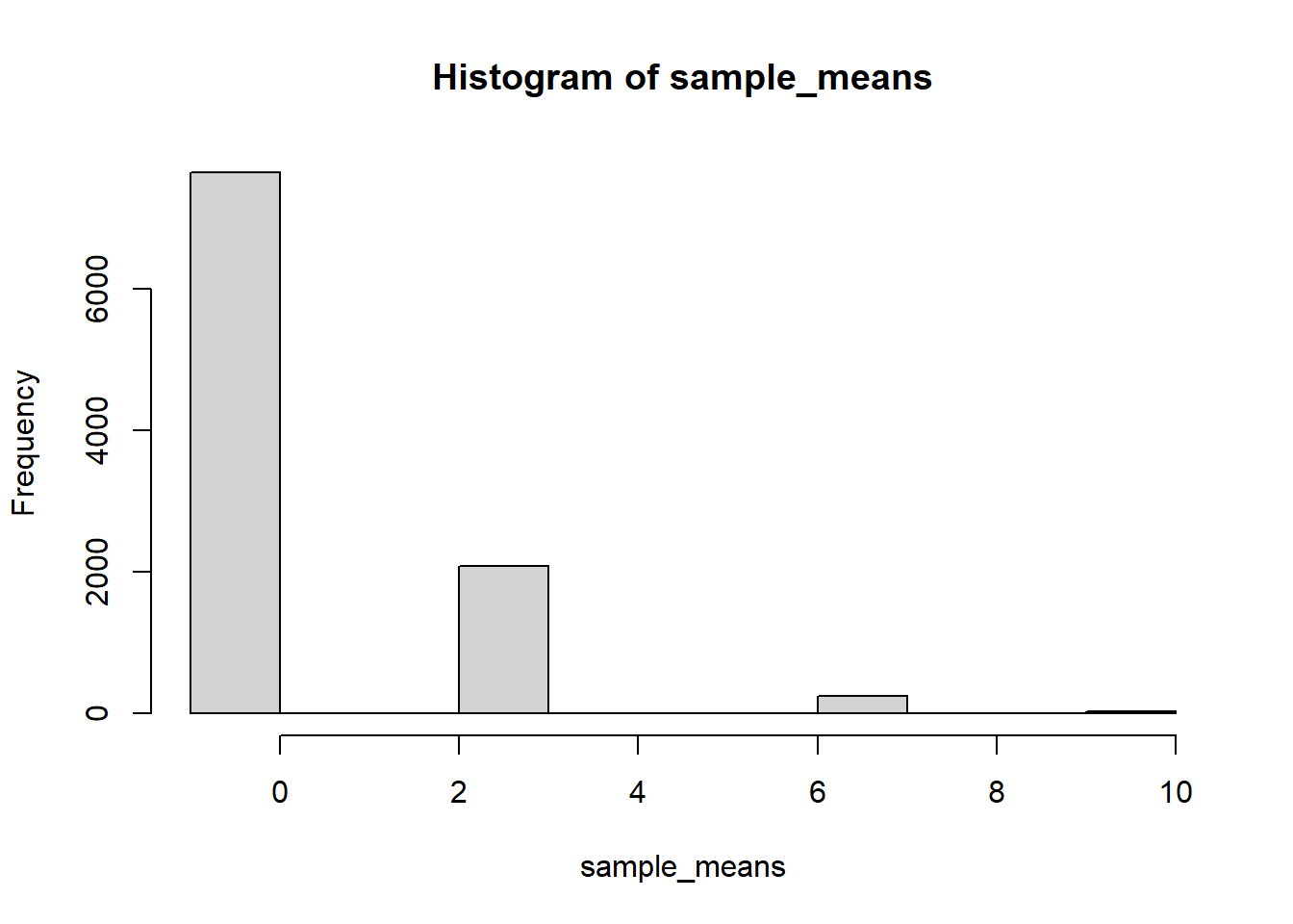
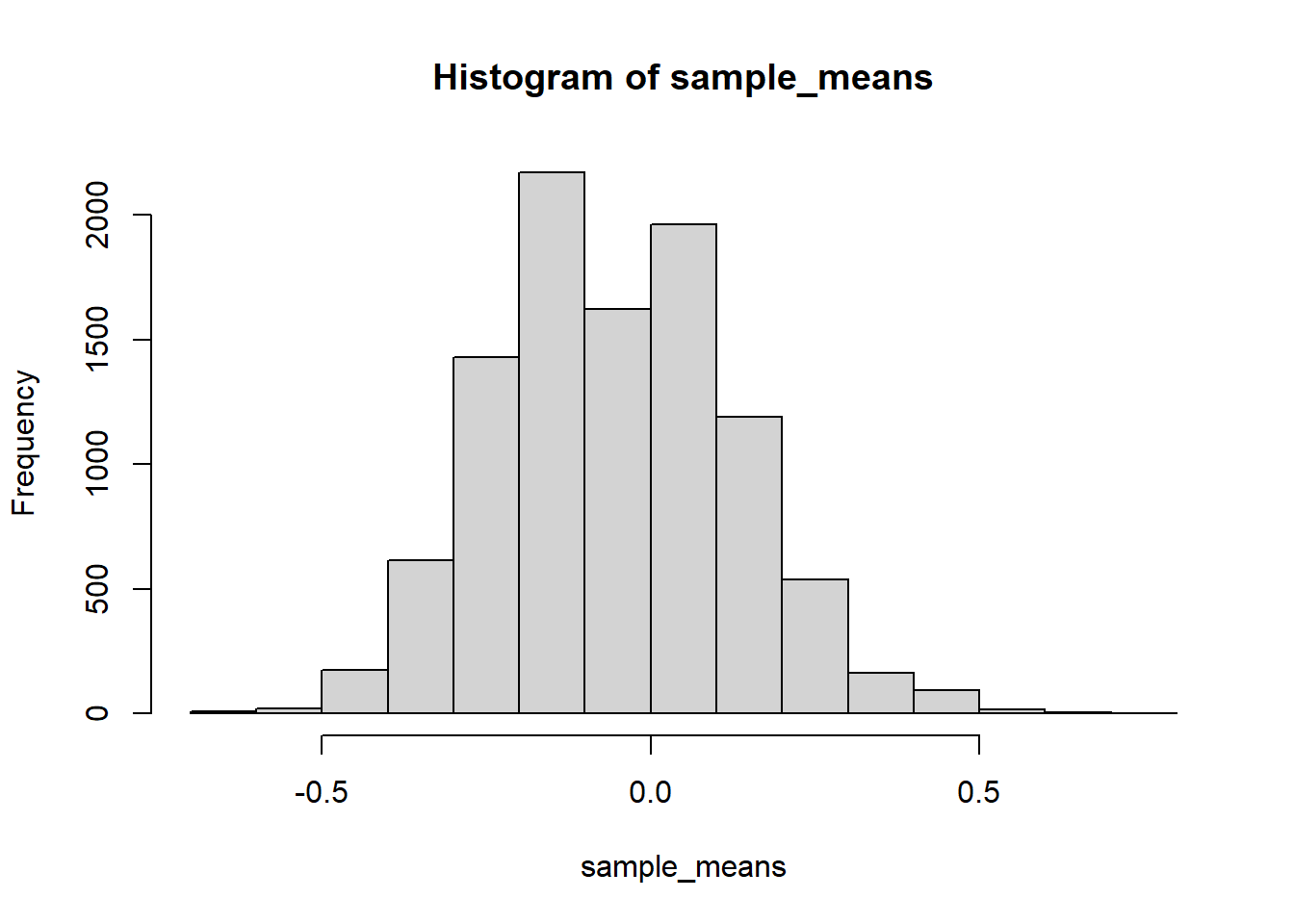
See simulation results in Colab notebook. Distribution does not look anything like Normal for \(n=10\) or \(n=100\). Shape of sample-to-sample distribution of sample means looks approximately Normal for \(n=1000\) (but there is still discrete versus continuous issue).
See simulation results in the Colab notebook. Your expected winnings are negative so the game is biased against you. In the long run, you lose, and the casino wins. So you don’t want to play in the long run. In the short run, there is a tradeoff: the more games you play the more chances you have to win at least once, and winning at least once can offset your losses. If you just play 10 games, the probability of winning at least once doesn’t offset your losses as effectively as when you play 100 games. In the short run, your probability of coming out ahead increases as you play more games, but eventually it starts to decrease with \(n\) as you play more and more games. (There is some weird discreteness in terms of number of possibilities that happens so the pattern is a little more complicated.) However, remember that \(\text{E}(\bar{X}_n)\) is negative for any \(n\). For example, consider \(n=35\). Suppose that every day you go to the casino and play 35 games. Then on about 60% of days you’ll end up ahead for that day. However, even though you end up ahead on more days than not, your winnings on the days you end up ahead are not enough to offset your losses on the other days. Over many days of 35 bets every day, you will lose about 35(2/38) = 1.84) dollars on average per day.
Assuming \(n=1000\) is large enough to the CLT to kick, \(\bar{X}_n\) has a Normal distribution with mean \(-2/38\) and SD \(5.76/\sqrt{1000}=\) 0.182. A value of 0 is \((0 - (-2/38))/0.182 = 0.289\) SDs above the mean. From the empirical rule, the probability will be between 0.5 and 0.31. Software (below) shows it’s 0.386.
Assuming \(n\) is large enough to the CLT to kick, \(\bar{X}_n\) has a Normal distribution with mean \(-2/38\) and SD \(5.76/\sqrt{n}\). We want to find \(n\) so that \(\text{P}(\bar{X}_n <0)= 0.99\). That is, we want 0 to be the 99th percentile. For a Normal distribution, the 99th percentile is 2.33 SDs above the mean. So we want to find \(n\) so that \(0 = -2/38 + 2.33(5.76/\sqrt{n})\). Solving for \(n\) gives \(n = (2.33(5.76)/(2/38))^2 = 64878\). (Roulette spins happen about once every minute at a casino. Even if the casino only has a single wheel with a single bet on each spin, the casino would easily clear more than the required number of bets in a day. Your bets are essentially free money for the casino.)
n =10N_samples =10000sample_means =vector(length = N_samples)for (i in1:N_samples) { x =sample(c(-1, 35), size = n, prob =c(37, 1) /38, replace =TRUE) sample_means[i] =mean(x)}hist(sample_means)
mean(sample_means)
[1] -0.04348
sd(sample_means)
[1] 1.834692
sum(sample_means >0) / N_samples
[1] 0.2357
n =100N_samples =10000sample_means =vector(length = N_samples)for (i in1:N_samples) { x =sample(c(-1, 35), size = n, prob =c(37, 1) /38, replace =TRUE) sample_means[i] =mean(x)}hist(sample_means)
mean(sample_means)
[1] -0.0559
sd(sample_means)
[1] 0.5723487
sum(sample_means >0) / N_samples
[1] 0.4938
n =1000N_samples =10000sample_means =vector(length = N_samples)for (i in1:N_samples) { x =sample(c(-1, 35), size = n, prob =c(37, 1) /38, replace =TRUE) sample_means[i] =mean(x)}hist(sample_means)
mean(sample_means)
[1] -0.0518968
sd(sample_means)
[1] 0.1815168
sum(sample_means >0) / N_samples
[1] 0.3963
1-pnorm(0, -2/38, 5.76/sqrt(1000))
[1] 0.3863095
qnorm(0.99)
[1] 2.326348
pnorm(0, -2/38, 5.76/sqrt(64878))
[1] 0.9900282
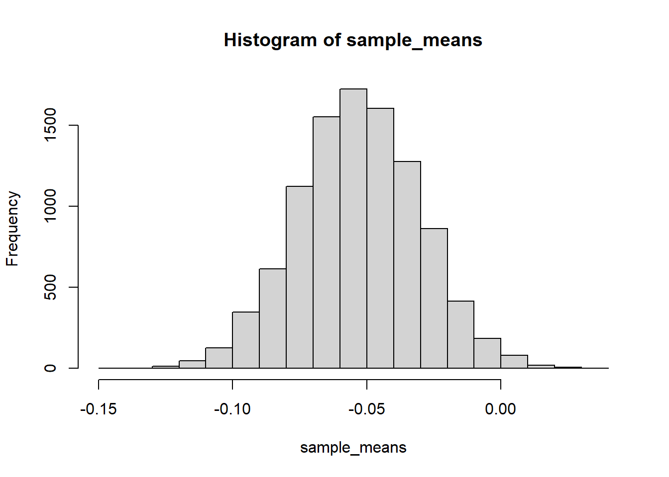
n =64878N_samples =10000sample_means =vector(length = N_samples)for (i in1:N_samples) { x =sample(c(-1, 35), size = n, prob =c(37, 1) /38, replace =TRUE) sample_means[i] =mean(x)}hist(sample_means)
mean(sample_means)
[1] -0.05282828
sd(sample_means)
[1] 0.02280221
sum(sample_means <0) / N_samples
[1] 0.9892
Problem 2
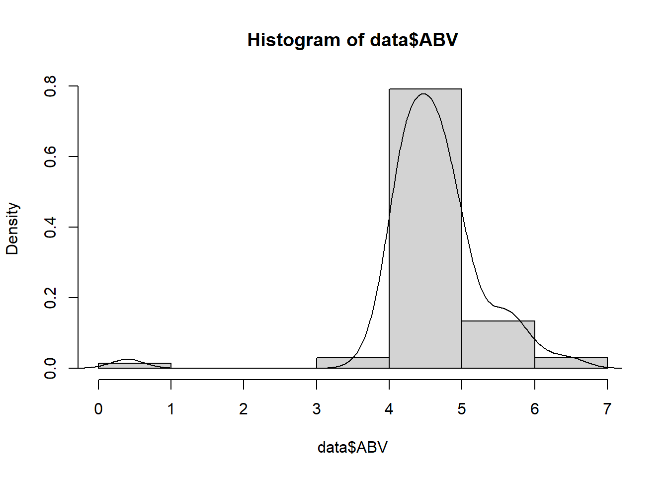
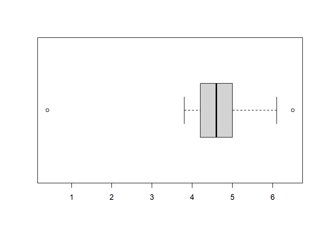
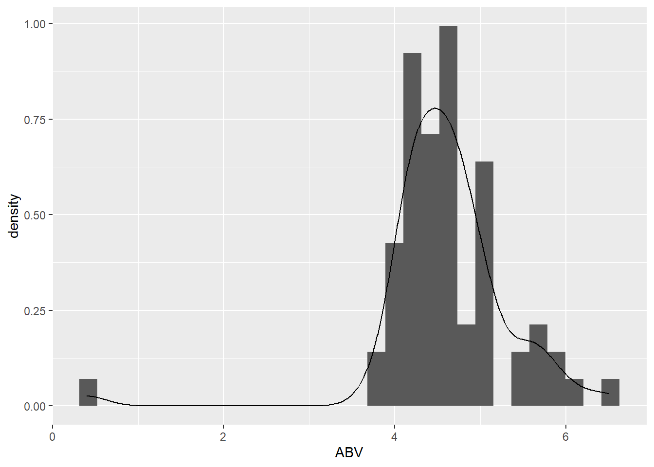
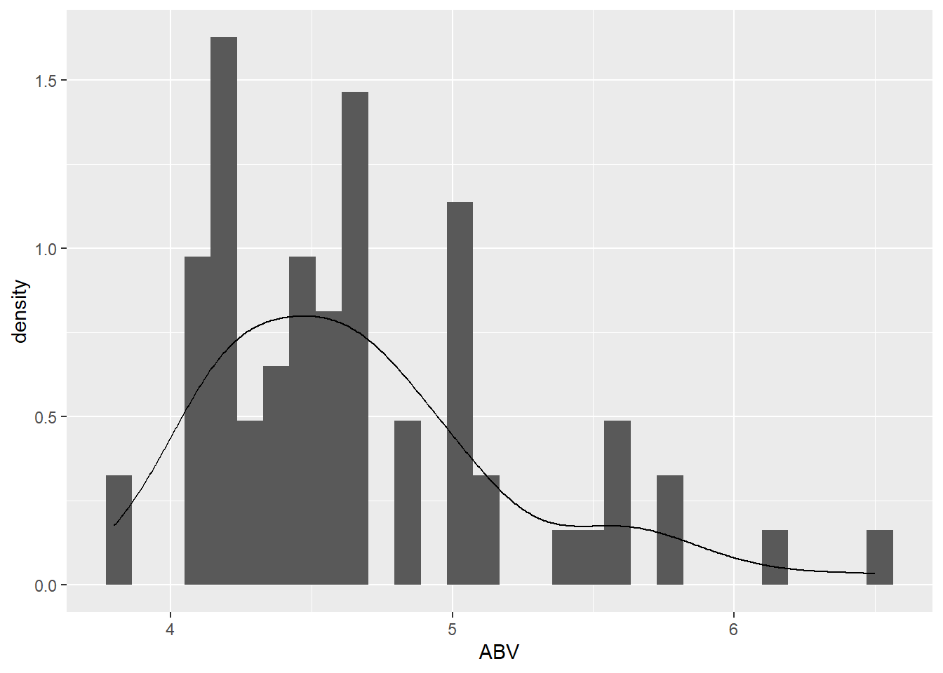
The standard measurement of the alcohol content of drinks is alcohol by volume (ABV), which is given as the volume of ethanol as a percent of the total volume of the drink. A report states that on average the ABV for beer is 4.5%. Is this true? In a sample of 67 brands of beer, the mean ABV is 4.61 percent and the standard deviation of ABV is 0.754 percent. Note: the data set and some R summaries are provided in Canvas so you can check your answers. But you should answer these questions by hand, using only the information provided here.
Use R to summarize the sample data. Then describe the main features in a sentence or two.
Compute an interpret a 95% confidence interval for the appropriate population mean.
Write a clearly worded sentence reporting your confidence interval in context.
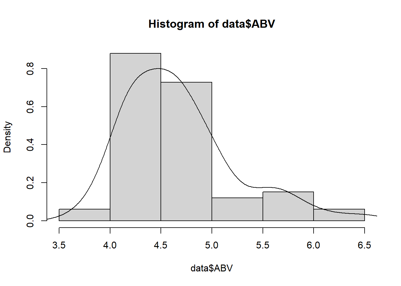
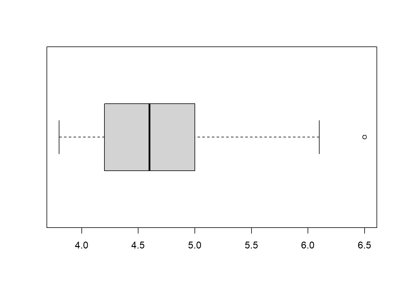
One of the brands of beer in the sample is O’Doul’s, a non-alcoholic beer. The ABV for O’Doul’s is 0.4 (it has a bit of alcohol.) Suppose O’Doul’s is removed from the data set. Compute the sample mean ABV of the remaining 66 brands. (You can do this with filter in tidyverse; see how I filtered the 2-week babies in the feeding length data.)
Continuing the previous part, compute the sample SD of ABV of the remaining 66 brands. Compare to the original sample mean; which mean is larger — with or without O’Doul’s? Explain briefly.
The sample SD of ABV of the remaining 66 brands is 0.55 percent. Compare to the original sample SD; which SD is larger — with or without O’Doul’s? Explain briefly.
Compute the 95% confidence interval based on the sample with O’Doul’s removed. Compute to the original interval, both in terms of center of the CI and its width. Explain briefly.
Based on the interval based on the sample with O’Doul’s removed, is 4.5% a plausible value of the parameter? Explain briefly.
Which of the analyses is more appropriate: with or without O’Doul’s? Explain your reasoning.
Solution
See below. The main features that stands out is the outlier. The sample mean is 4.61 and the sample SD is 0.754.
The SE of \(0.754/\sqrt{67}= 0.092\) measures the sample-to-sample variability of sample mean ABV over many samples of 67 brands of beer each. The 95% CI is \(4.61 \pm 2 × 0.092 \Rightarrow 4.61 \pm 0.184 \Rightarrow [4.42, 4.79].\)
We estimate with 95% confidence that the population mean ABV for brands of beer is between 4.42 and 4.79 percent.
The outlier pulled the mean down, so the mean is larger without it.
The sample SD of ABV was larger with O’Doul’s; the outlier pulled up the average distance from the mean.
O’Doul’s was bringing down the mean, so removing it increase the sample mean and increases the center of the confidence interval. Removing O’Doul s results in a smaller sample SD, and a narrower CI.
Technically, no since the value 4.5 percent lies outside the CI. (Though this we would really want a p-value to measure the strength of the evidence; here we’re basically just saying that the p-value is less than 0.05.)
In general, EXCLUDING OUTLIERS WITHOUT A COMPELLING REASON IS BAD. However, in this case the population we are interested in is brands of beer, probably meaning beer with actual alcohol in it. So it makes sense to only consider a sample of alcoholic beers, and so I think the more appropriate analysis with the non-alcoholic beer excluded.
Warning: The dot-dot notation (`..density..`) was deprecated in ggplot2 3.4.0.
ℹ Please use `after_stat(density)` instead.
`stat_bin()` using `bins = 30`. Pick better value with `binwidth`.
t.test(data$ABV, mu =4.5)
    One Sample t-test

data:  data$ABV
t = 1.199, df = 66, p-value = 0.2348
alternative hypothesis: true mean is not equal to 4.5
95 percent confidence interval:
 4.426531 4.794364
sample estimates:
mean of x
 4.610448
Excluding outlier
data = data |>filter(!(Brand =="O'Doul's"))summary(data$ABV)
   Min. 1st Qu.  Median    Mean 3rd Qu.    Max.
  3.800   4.200   4.600   4.674   5.000   6.500
sd(data$ABV)
[1] 0.5480906
data |>summarize(n =n(),mean =mean(ABV),sd =sd(ABV),min =fivenum(ABV)[1],Q1 =fivenum(ABV)[2],median =fivenum(ABV)[3],Q3 =fivenum(ABV)[4],max =fivenum(ABV)[5])
   n     mean        sd min  Q1 median Q3 max
1 66 4.674242 0.5480906 3.8 4.2    4.6  5 6.5
`stat_bin()` using `bins = 30`. Pick better value with `binwidth`.
t.test(data$ABV, mu =4.5)
    One Sample t-test

data:  data$ABV
t = 2.5827, df = 65, p-value = 0.01206
alternative hypothesis: true mean is not equal to 4.5
95 percent confidence interval:
 4.539505 4.808980
sample estimates:
mean of x
 4.674242
Problem 4
(I had much longer instructions written, but I think they weren’t helpful. If you have questions about how the applet is working, don’t hesitate to ask.)
You are going to use a simulation applet that randomly generates confidence interals for a population mean to help you understand some ideas. The applet calculates a confidence interval for each set of randomly generated data.
In the box for “Statistic” select means “Means”.
In the box next to “Method” select “t”.
Start with “Number of intervals” equal to 1 at first to see what is happening, but then change it to lots.
Experiment with different simulations; be sure to change
Distribution
Population Mean
Population SD
Sample size
Confidence level
Then write a paragraph or two or some bullet points of your main observations. Based on this applet, what can you say about how confidence intervals work? How does changing the inputs affect the confidence intervals and the Results?
Solution
Simulated coverage level is generally close to confidence level, unless sample size is small and population is not Normal
Increasing population SD makes the intervals wider
Increasing the sample size make the intervals narrower
Increasing the confidence level makes the intervals wider
Since sample means are unbiased estimators of the population mean, when the population mean changes, the sample means follow it.