10 Percentiles

Example 10.1 Maggie and Seamus are babies who have just turned one. At their one-year visits to their pediatrician:

Maggie is 76cm tall and in the 75th percentile of height for girls.
Seamus is 72cm tall and in the 10th percentile of height for boys.

Explain what these percentiles mean.

A distribution is characterized by its percentiles.
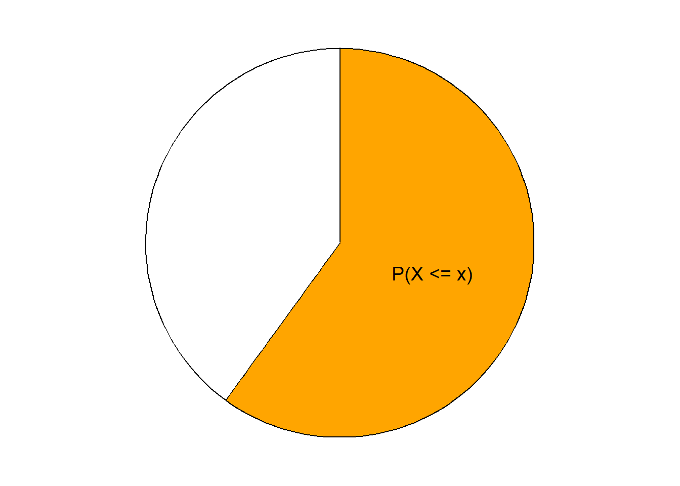
Roughly, the value $x$ is the $p$th percentile (a.k.a. quantile) of a distribution of a random variable $X$ if $p$ percent of values of the variable are less than or equal to $x$: $\text{P}(X\le x) = p$.
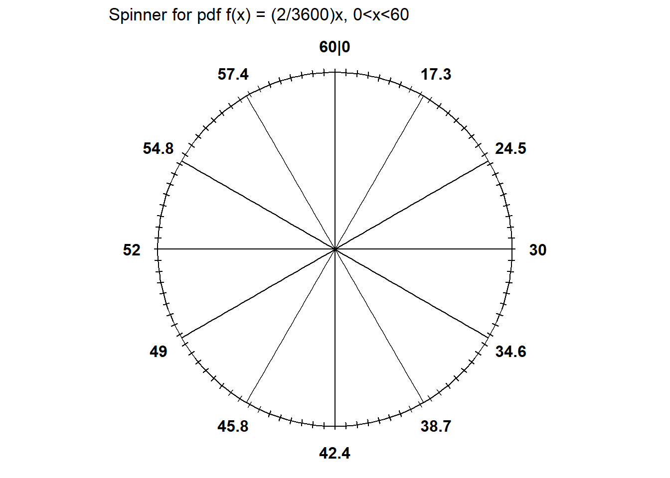
Any distribution can be represented by a spinner. A spinner basically describes a distribution by specifying all the percentiles. For example,
- The 25th percentile goes 25% of the way around the axis (at “3 o’clock”)
- The 50th percentile goes 50% of the way around the axis (at “6 o’clock”)
- The 75th percentile goes 75% of the way around the axis (at “9 o’clock”)

10.1 Cumulative Distribution Functions

Roughly, the value $x$ is the $p$th percentile of a distribution of a random variable $X$ if $p$ percent of values of the variable are less than or equal to $x$: $\text{P}(X\le x) = p$.
The cumulative distribution function (cdf) of a random variable fills in the blank for any given $x$: $x$ is the (blank) percentile. That is, for an input $x$, the cdf outputs $\text{P}(X\le x)$.
The cumulative distribution function (cdf) of a random variable $X$ is the function, $F_X$ defined by $F_X(x) = \text{P}(X\le x)$. A cdf is defined for all real numbers $x$ regardless of whether $x$ is a possible value of $X$.

Example 10.2 Continuing Example 9.2 where Regina’s arrival time $X$ (minutes after noon) has pdf \[ f_X(x) = (2/3600) x, \qquad 0<x<60. \] Let $F_X$ be the cdf of $X$.

Compute and interpret $F_X(15)$.
Compute and interpret $F_X(45)$.
Compute and interpret $F_X(45) - F_X(15)$.
Compute $F_X(-0.2)$
Compute $F_X(70)$
Find the cdf of $X$.

Example 10.3 Let $X$ be the number of heads in 3 flips of a fair coin.

Find the pmf of $X$ and sketch a plot of it.
Find the cdf of $X$ and sketch a plot of it.
Let $Y$ be the number of tails in 3 flips of a fair coin. Find the cdf of $Y$.

A cdf is defined for all values of $x$, regardless if $x$ is a possible value of the RV.
A cdf is a non-decreasing function: if $x_1 \le x_2$ then $F_X(x_1)\le F_X(x_2)$.
A cdf approaches 0 as the input approaches $-\infty$: $\lim_{x\to-\infty}F_X(x) = 0$
A cdf approaches 1 as the input approaches $\infty$: $\lim_{x\to\infty}F_X(x) = 1$
The cdf of a discrete random variable is a step function.
- The steps occur at the possible values of the random variable.
- The height of a particular step corresponds to the probability of that value, given by the pmf.
The cdf of a continuous random variable is a continuous function.
- The cdf of a continuous random variable is obtained by integrating the pdf, so
- The pdf of a continuous random variable is obtained by differentiating the cdf \[ F_X' = f_X \qquad \text{if $X$ is continuous} \]
For any random variable $X$ with cdf $F_X$ \[ F_X(b) - F_X(a) = \text{P}(a<X \le b) \] Whether the inequalities in the above event are strict ($<$) or not ($\le$) matters for discrete random variables, but not for continuous.
Random variables $X$ and $Y$ have the same distribution if their cdfs are the same, that is, if $F_X(u) = F_Y(u)$ for all $u$.
That is, two random variables have the same distribution if all the percentiles are the same.

10.2 Quantile functions

The quantile function (essentially the inverse cdf) fills in the following blank for a given $p\in[0, 1]$: the $100p$th percentile is (blank).

Example 10.4 Continuing Example 9.2 where Regina’s arrival time $X$ (minutes) had pdf \[ f_X(x) = (2/3600)x, \qquad 0<x<60. \]

Find the median (i.e., 50th percentile) of $X$.
Find the 25th percentile of $X$.
Find the quantile function of $X$.
Construct a spinner for simulating values of $X$ according to its distribution.

For a continuous random variable $X$ with cdf $F_X$, the quantile function $Q_X$ is the inverse of the cdf, $Q_X(p) = F_X^{-1}(p)$.
The quantile function (essentially the inverse cdf) fills in the following blank for a given $p\in[0, 1]$: the $100p$th percentile is (blank).
For example, evaluating the quantile function at $p=0.25$ outputs the 25th percentile.
The quantile function can be used to create a spinner for a distribution. Basically, the values on the outside boundary of the spinner are scaled based on the quantile function (which is determined by the cdf). Intervals corresponding to regions of higher density (“more likely”) values are stretched out on the spinner boundary; intervals corresponding regions of lower density (“less likely” values) are shrunk.

Universality of the Uniform (or “one spinner to rule them all”). Let $F$ be a cdf and $Q$ its corresponding quantile function. Let $U$ have a Uniform(0, 1) distribution and define the random variable $X=Q(U)$. Then the cdf of $X$ is $F$.
Universality of the uniform might look complicated but all it basically says is that you can construct a spinner by putting the 25th percentile 25% of the way around, the 75th percentile 75% of the way around, etc.
Actually, universality of the uniform says we don’t have to create a new spinner. We can just spin the Uniform(0, 1) spinner and transform each resulting value by plugging it into the quantile function.

N_rep = 10000

u = runif(N_rep, 0, 1)

x = 60 * sqrt(u)

hist(x,
     freq = FALSE,
     main = "")

Figure 10.5: Simulated values of $X$ with the pdf in Example 9.2.