9.2 Cointegration
It is very common to analyze the cointegration (short-run and long-run relationship) between two or more time-series using so called Error Correction Model (ECM)
Assuming that single RHS variable \(x_t\) is exogenous, ECM can be obtained as reparametrized ARDL\((1,1)\) by replacements \(\lambda=\beta_1+\beta_2\) and \(\gamma=\beta_3-1\)
\[\begin{equation} \begin{aligned} y_t&= \beta_0+\beta_1 x_t + \beta_2 x_{t-1} + \beta_3 y_{t-1} + u_t \\ \Delta y_t + y_{t-1}&= \beta_0+\beta_1 (\Delta x_t + x_{t-1})+ \beta_2 x_{t-1} + \beta_3 y_{t-1} + u_t \\ \Delta y_t&= \beta_0+ \beta_1 \Delta x_t + (\beta_1 + \beta_2) x_{t-1} + (\beta_3 - 1) y_{t-1} + u_t \\ \Delta y_t&=\beta_0+\beta_1 \Delta x_t+\lambda x_{t-1}+\gamma y_{t-1}+u_t \end{aligned} \tag{9.14} \end{equation}\]
\(~~~~~~~\)where \(\Delta y_t\) and \(\Delta x_t\) are first differences of \(y_t\) and \(x_t\), while \(x_{t-1}\) and \(y_{t-1}\) are lagged values of \(y_t\) and \(x_t\)
Equation (9.14) can be additionally rearranged in the following way \[\begin{equation} \begin{aligned} \Delta y_t&=\beta_0+\beta_1 \Delta x_t+\gamma \bigg( y_{t-1}+\frac{\lambda}{\gamma}x_{t-1} \bigg) +u_t \\ \Delta y_t&=\beta_0+\underbrace{\beta_1}_{short-run} \Delta x_t-(\underbrace{1-\beta_3}_{correction}) \underbrace{ \bigg( y_{t-1}-\underbrace{\frac{\beta_1+\beta_2}{1-\beta_3}}_{long-run}x_{t-1} \bigg) }_{disequilibrium}+u_t \end{aligned} \tag{9.15} \end{equation}\]
Parameter \(\gamma\) is expected to be negative due to correction of short-run disequilibrium in every period for \((1-\beta_3)100\%\). That’s why parameter \(\gamma\) is known as speed of adjustment or correction
The last equation in (9.14) provides the same information as ARDL(\(1,1\)) model - the first equation in (9.14)
Short-run effect is \(\beta_1\)
Speed of adjustment is \(-\gamma=-(\beta_3-1)=(1-\beta_3)\)
Long-run effect is \(\frac{\lambda}{-\gamma}=\frac{\beta_1+\beta_2}{1-\beta_3}\)
ECM can be estimated in one step as a single equation as in (9.14)
Alternative is two step estimation approach proposed by Engle and Granger

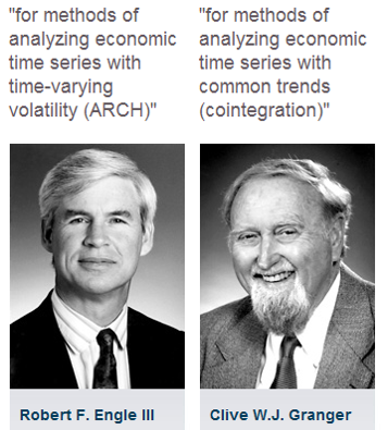
FIGURE 9.1: Nobel Prize winners in 2003 for their contribution in time-series econometrics
Engle-Granger approach is a two step approach in finding cointegration between two time-series
Step \(1)\) Assuming that both time-series \(y_t\) and \(x_t\) are nonstationary, a static model between two nonstationary time-series is estimated in the first step \[\begin{equation} \begin{array}{c} y_t=\beta_0+\beta_1 x_t+u_t\\ y_t \sim I(1) \\ x_t \sim I(1) \\ u_t\sim I(0) \\ \end{array} \tag{9.16} \end{equation}\]
If the error terms of the static model \(u_t\) are stationary, or at least the lower integration order than \(y_t\) and \(x_t\), we conclude that cointegration exist (the null hypothesis of the ADF test of the residuals is rejected).
Step \(2)\) If cointegration exist, meaning that two time-series share a long-term equilibrium relationship while deviations from this equilibrium in the short-term are corrected over time, ECM is estimated in the second step \[\begin{equation} \begin{array}{c} \Delta y_t=\alpha_0+\alpha_1 \Delta x_t+\gamma \widehat{u}_{t-1}+e_t \\ \Delta y_t \sim I(0)\\ \Delta x_t \sim I(0) \\ \widehat{u}_{t-1} \sim I(0) \\ \end{array} \tag{9.17} \end{equation}\]
\(~~~\) where \(\widehat{u}_{t-1}\) are lagged residuals from a static model obtained as \(\widehat{u}_{t-1}=y_{t-1}-\beta_0-\beta_1 x_{t-1}\)
If cointegration exist, it means that the time-series \(y_t\) and \(x_t\) are related in both the short-run and the long-run, assuming the strict exogeneity of \(x_t\) (variable \(x_t\) causes \(y_t\) but not the other way around, which implies that time-series \(x_t\) and error terms \(u_t\) are independent), and hence a static model presents the equilibrium or cointegration equation, while the ECM presents short-run equation which also includes the correction of short-run disequilibrium.
Therefore, parameter \(\beta_1\) in the static model (9.16) presents the lon-run effect, parameter \(\alpha_1\) in the ECM presents the short-run effect, while parameter \(\gamma\) presents the correction of disequilibrium (speed of adjustment)
However, if cointegration does not exist it means that time-series \(x_t\) and \(y_t\) are related only in the short-run, which means that a static model is spurious (there is no long-run relationship), and instead of the ECM, the model in the first differences should be estimated \[\begin{equation} \Delta y_t=\alpha_0+\alpha_1 \Delta x_t+e_t \tag{9.18} \end{equation}\]
Parameter \(\alpha_1\) in the model (9.18) is the short-run effect
Short-run model (9.18) is the special case of the ECM (9.17) when \(\gamma=0\)
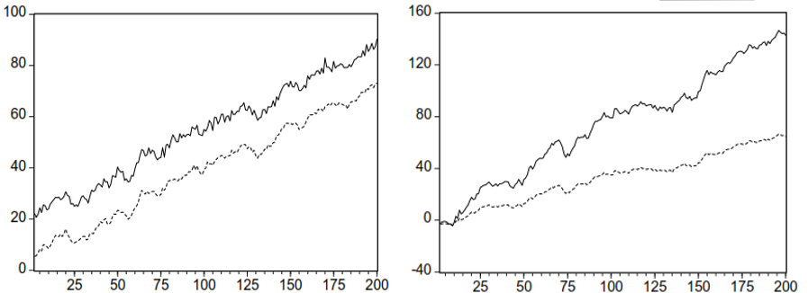
Cointegration exist only if time-series don’t drift apart from each other, as illustrated on the figure

FIGURE 9.2: Cointegrated and non-cointegrated time-series
growth rate and the production volume from the data frame indicators as a single time-series objects. Display both time-series growth and production on a grid with \(2\) columns and \(1\) row. Using the ur.df() command from the urca package, perform ADF test in the levels and in the first differences on growth and production to check the order of integration \(I(d)\). If both time-series are nonstationary and with the same integration odrder, e.g. \(I(1)\) or \(I(2)\), compute the ADF test in the levels of residuals from the static model (for that purpose first extract residuals from a static model using command resid() and latter compute ADF test in the levels type=“none”). If cointegration exist estimate error correction model ecm using dynlm() command from the dynlm package. Within dynlm() command, the first differences are computed using the difference operator d() and the lagged values are computed using lag operator L(). Present the results of the static model and ecm in a single table using modelsummary() command. Determine the short-run effect, the long-run effect and the speed of adjustment.
Solution
Copy the code lines below to the clipboard and paste them into an R Script file opened in RStudio. In this example ADF test is performed several times to check (non)stationarity of the growth, the production, and the residuals from the static model. Non rejection of the ADF null hypothesis in the levels and it’s rejection in the first differences for both time-series, indicates that growth and production are nonstationary in the levels, but stationary in the first differences. Therefore, both time-series are integrated of the same order \(I(1)\). However, residuals from the static model are stationary in the levels (ADF null hypothesis is rejected), which means they are integrated of order zero \(I(0)\). Following table summarizes the results of ADF tests.
| Time-series | ADF test in the levels | ADF in the first differences |
|---|---|---|
| growth | \(~~~~~~~~-1.711\) | \(~~~~~~~~-4.768^{***}\) |
| production | \(~~~~~~~~-2.065\) | \(~~~~~~~~-5.684^{***}\) |
| residuals | \(~~~~~~~~-2.919^{***}\) |
growth and productioin exist. Therefore, we proceed with ecm.
# Separating "growth" and "production" from a data frame "indicators" as a single time-series objects
growth=ts(indicators[,"growth"],frequency=4,start=c(2000,1))
production=ts(indicators[,"production"],frequency=4,start=c(2000,1))

# Plotting the two time-series side by side on a grid with 2 columns and 1 row
layout(matrix(c(1:2), nrow=1))
ts.plot(growth, main="GDP growth of China", xlab="",ylab="growth rate in %")
ts.plot(production, main="Production of China", xlab="", ylab="volume index")

library(urca) # loading "urca" package (required only in a new session)
# Performing ADF test in the levels and in the first differences for "growth"
# Time-series oscillates around a non-zero mean but does not exhibit any trending behavior (type="drift")
summary(ur.df(growth, type="drift", selectlags="AIC"))  # ADF test in the levels with drift
summary(ur.df(diff(growth), type="drift", selectlags="AIC"))  # ADF test in the first differences with drift

# Performing ADF test in the levels and in the first differences for "production"
summary(ur.df(production, type="drift", selectlags="AIC"))  # ADF test in the levels with drift
summary(ur.df(diff(production), type="drift", selectlags="AIC"))  # ADF test in the first differences with drift

# Extracting the "residuals" from the "static" model as a single time-series object
residuals=ts(resid(static),frequency=4,start=c(2000,1))
# Performing ADF test in the levels for the "residuals" without drift and without trend (type="none")
summary(ur.df(residuals, type="none", selectlags="AIC"))

# Estimating ECM proposed by Engle and Granger
ecm=dynlm(d(growth)~d(production)+L(residuals))

# Presenting the results of both models  ("static" and "ecm")
modelsummary(list("Static (long-run)"=static,"ECM"=ecm),stars=TRUE,fmt=4)

# Long-run effect is the second coefficient from the "static" model
coef(static)[2]

# Short-run effect is the second coefficient from the "ecm"
coef(ecm)[2]

# Speed of adjustment is the third coefficient from the "ecm"
coef(ecm)[3]
\(~~~\)
growth and production, implying that two time-series are related only in the short-run (but not in the long-run). In that case residuals from the static model would be nonstationary and integrated of order one \(I(1)\) just like growth and production. In this scenario only short-run model short should be estimated.
Solution
Copy the code lines below to the clipboard and paste them into an R Script file opened in RStudio. When cointegration does not exist, only short-run model is required. Short-run model includes only the first differences of both time-series. In this example the short-run effect is \(0.0498\) and not statistically significant.# Estimating short-run model only named as "short"
short=dynlm(d(growth)~d(production))
# Presenting the results of the "short" model
modelsummary(list("Short-run model"=short),stars=TRUE,fmt=4)
# Short-run effect is the second coefficient from the "short" model
coef(short)[2]\(~~~\)