5.1 OLS method
- Based on the following hypothetical example, the OLS method will be discussed in detail, along with it’s assumptions and properties
Hypothetical example: linear dependence between weekly consumption (variable \(y\)) and weekly income (variable \(x\)) is analyzed in a population of \(60\) households (TABLE 5.1). For the same reason households are divided into \(10\) groups with the same income level (both variables are measured in USD).
| \(~Income~\) | \(~~~~~~~~\) | \(~~~~~~~~\) | \(~~~~~~~~\) | \(~~~~~~~~\) | \(~~~~~~~~\) | \(~~~~~~~~\) | \(~~~~~~~~\) | \(~E(y|x_i)~\) |
|---|---|---|---|---|---|---|---|---|
| 80 | 55 | 60 | 65 | 70 | 75 | NA | NA | 65 |
| 100 | 65 | 70 | 74 | 80 | 85 | 88 | NA | 77 |
| 120 | 79 | 84 | 90 | 94 | 98 | NA | NA | 89 |
| 140 | 80 | 93 | 95 | 103 | 108 | 113 | 115 | 101 |
| 160 | 102 | 107 | 110 | 116 | 118 | 125 | NA | 113 |
| 180 | 110 | 115 | 120 | 130 | 135 | 140 | NA | 125 |
| 200 | 120 | 136 | 140 | 144 | 145 | NA | NA | 137 |
| 220 | 135 | 137 | 140 | 152 | 157 | 160 | 162 | 149 |
| 240 | 137 | 145 | 155 | 165 | 175 | 189 | NA | 161 |
| 260 | 150 | 152 | 175 | 178 | 180 | 185 | 191 | 173 |
Conditional expectation \(E(y|x_i)\) is average weekly consumption conditioned by the income level, i.e. conditional mean linearly depends on income \(x\) \[\begin{equation} E(y|x_i)=\beta_0+\beta_1x_i \tag{5.1} \end{equation}\]
Inserting a values of \(E(y|x_i)\) and \(x_i\) in the EQUATION (5.1) the system of \(10\) equations holds
\[\begin{equation} \begin{aligned} 65=&\beta_0+\beta_1 80 \\ 77=&\beta_0+\beta_1 100 \\ & \vdots \\ 173=&\beta_0+\beta_1 260 \end{aligned} \tag{5.2} \end{equation}\]
From any two equations of the system (5.2) it’s easy to conclude that \(\beta_0=17\) and \(\beta_1=0.6\)
Not surprisingly, straight line passes through the conditional means due to linear dependence, which is known as population regression line
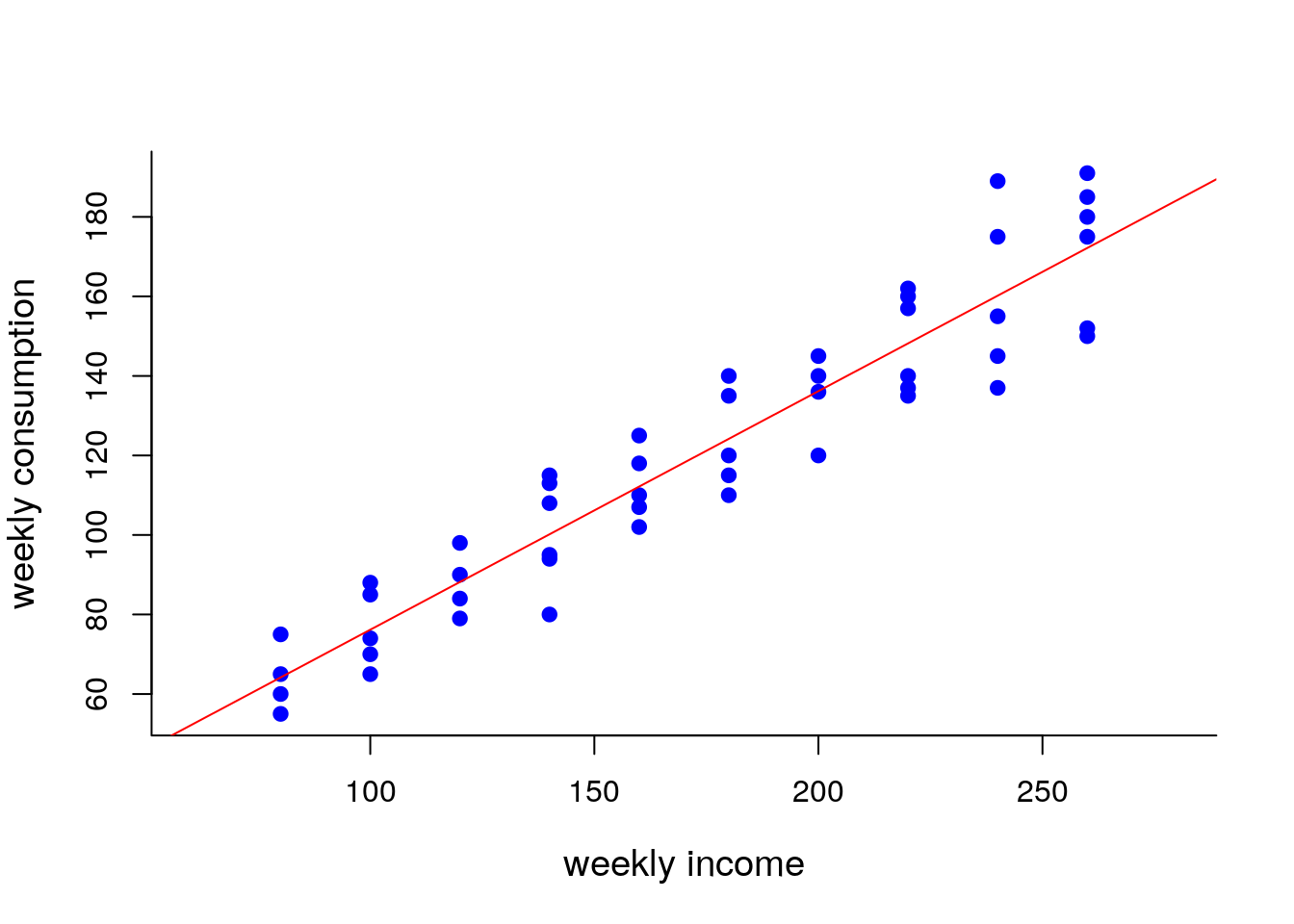
FIGURE 5.1: Population regression line
\(~~~\)
Weekly consumption for each individual household \(y_i\) differs from the conditional mean \[\begin{equation} y_i-E(y|x_i)=u_i \tag{5.3} \end{equation}\]
Inserting EQUATION (5.1) into EQUATION (5.3) we get population regression model \[\begin{equation} y_i=\beta_0+\beta_1x_i+u_i \tag{5.4} \end{equation}\]
Disturbance \(u_i\) is an error term which presents a random variable with zero conditional mean for every income level \[\begin{equation} E(u|x_i)=E(u_i)=0 \tag{5.5} \end{equation}\]
It is additionally assumed that conditional variance of error terms should be finite and constant (equal across all income levels)
\[\begin{equation} Var(u|x_i)=Var(u_i)=\sigma^2 \tag{5.6} \end{equation}\]
- Identities \(E(u|x_i)=E(u_i)\) and \(Var(u|x_i)=Var(u_i)\) holds if variable \(x\) is not random but fixed. Otherwise, both random variables \(u\) and \(x\) should be independent, i.e. not correlated (\(x\) does not give us any information about \(u\))
\[\begin{equation} Cov(u_i,x_i)=0 \tag{5.7} \end{equation}\]
- Moreover, error terms should be independently distributed across income levels
\[\begin{equation} Cov(u_i,u_j)=0~~~~~i \ne j \tag{5.8} \end{equation}\]
- Thus, error terms \(u_i\) are independently distributed random variables with mean zero and equal variances. Random variables which have equal means and equal variances are identically distributed.
\[\begin{equation} u_i \sim i.i.d.(0, \sigma^2) \tag{5.9} \end{equation}\]
| \(~Income~\) | \(~~~~~~~\) | \(~~~~~~~\) | \(~~~~~~~\) | \(~~~~~~~\) | \(~~~~~~~\) | \(~~~~~~~\) | \(~~~~~~~\) | \(~E(u|x_i)~\) | \(~Var(u|x_i)~\) |
|---|---|---|---|---|---|---|---|---|---|
| 80 | -10 | -5 | 0 | 5 | 10 | NA | NA | 0 | 50 |
| 100 | -12 | -7 | -3 | 3 | 8 | 11 | NA | 0 | 66 |
| 120 | -10 | -5 | 1 | 5 | 9 | NA | NA | 0 | 46 |
| 140 | -21 | -8 | -6 | 2 | 7 | 12 | 14 | 0 | 133 |
| 160 | -11 | -6 | -3 | 3 | 5 | 12 | NA | 0 | 57 |
| 180 | -15 | -10 | -5 | 5 | 10 | 15 | NA | 0 | 117 |
| 200 | -17 | -1 | 3 | 7 | 8 | NA | NA | 0 | 82 |
| 220 | -14 | -12 | -9 | 3 | 8 | 11 | 13 | 0 | 112 |
| 240 | -24 | -16 | -6 | 4 | 14 | 28 | NA | 0 | 311 |
| 260 | -23 | 21 | 2 | 5 | 7 | 12 | 18 | 0 | 2017 |
Population is often finite but unknown or infinite (when dealing with time-series data) so the error terms \(u_i\) are also unknown as well as parameters \(\beta_0\) and \(\beta_1\). However, population parameters and error terms can be easily estimated by using sample data of size \(n\).
Selection of simple random sample SRS requires that error terms are identically distributed (with zero mean and constant variance) and independently distributed (zero covariances between themselves)
|
|
TABLE 5.3 conclude which variable is random and which one is not random in repeated sampling?
Solution
In repeated sampling, variable \(x\) (weekly income) has the same values accros households, and thus, \(x\) is fixed variable within cross-sectional data. In contrast, variable \(y\) (weekly consumption) takes different values accros households, meaning it is a random variable.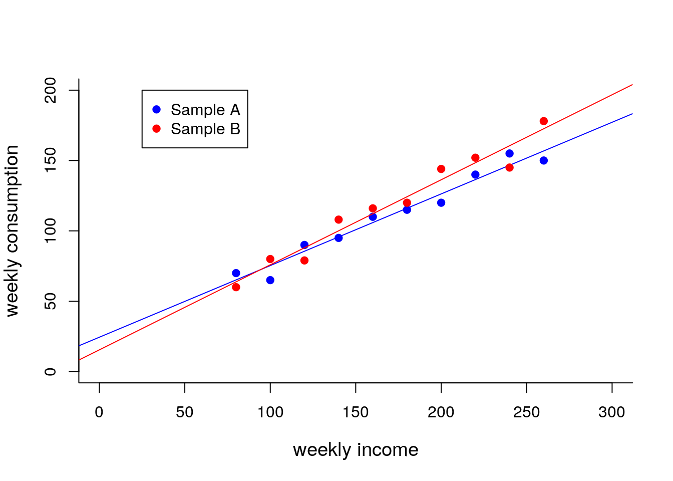
FIGURE 5.2: Sample regression lines
\(~~~\)
- Any random variable has a certain probability distribution. If random variable \(y\) is continuous it is assumed to be normally distributed. It implies that error terms, which are also random variables, should be normally distributed.
Unknowns, which are being estimated by using sample data, are usually denoted with “hats”, and thus \[\begin{equation} y_i=\hat{\beta}_0+\hat{\beta}_1x_{i,1}+\hat{\beta}_2x_{i,2}+\cdots+\hat{\beta}_kx_{i,k}+\hat{u}_i \tag{5.10} \end{equation}\] represents sample regression model with \(k\) variables on the RHS
Sample regression model based on \(n\) observations (\(i=1,2,...,n\)) and \(k\) independent variables (\(j=1,2,...,k\)) in matrix notation \[\begin{equation}\underbrace{\begin{bmatrix} y_1 \\ y_2 \\ \vdots \\ y_n\end{bmatrix}}_{y}=\underbrace{\begin{bmatrix} 1 & x_{1,1} & x_{1,2} & \cdots & x_{1,k} \\ 1 & x_{2,1} & x_{2,2} & \cdots & x_{2,k} \\ \vdots & \vdots \\ 1 & x_{n,1} & x_{n,2} & \cdots & x_{n,k} \end{bmatrix}}_{x} \underbrace{\begin{bmatrix} \hat{\beta}_0 \\ \hat{\beta}_1 \\ \vdots \\ \hat{\beta}_k \end{bmatrix}}_{\hat{\beta}}+\underbrace{\begin{bmatrix} \hat{u}_1 \\ \hat{u}_2 \\ \vdots \\ \hat{u}_n \end{bmatrix}}_{\hat{u}} \tag{5.11} \end{equation}\]
Estimated error terms are called residuals, and the residual sum of squares \(\displaystyle \sum_{i=1}^{n}\hat{u}_i^2~\) is a vector function
\[\begin{equation} \hat{u}^{T}\hat{u}=(y-x\hat{\beta})^{T}(y-x\hat{\beta})=y^{T}y-2\hat{\beta}^{T}x^{T}y+\hat{\beta}^{T}x^{T}x\hat{\beta} \tag{5.12} \end{equation}\]
Residual sum of squares (RSS) is minimized with respect to vector \(\hat{\beta}\) \[\begin{equation} \frac{\partial \hat{u}^{T}\hat{u}}{\partial \hat{\beta}}=-2x^{T}y+2x^{T}x\hat{\beta}=0 \tag{5.13} \end{equation}\]
From a first order condition we get a system of normal equations \[\begin{equation} x^{T}x\hat{\beta}=x^{T}y \tag{5.14} \end{equation}\]
The solution of the system in matrix form is OLS formula \[\begin{equation} \hat{\beta}=(x^{T}x)^{-1}x^{T}y \tag{5.15} \end{equation}\]
- Firstly, vector \(\hat{\beta}\) of length \((k+1)\) is calculated, and afterwords a residuals vector \(\hat{u}\) of lenght \(n\) is calculated by
\[\begin{equation} \begin{aligned} \hat{u}&=y-\hat{y} \\ &=y-x \hat{\beta} \end{aligned} \tag{5.16} \end{equation}\]
Solution in EQUATION (5.15) exist if there is inverse of \((x^{T}x)\), i.e. columns of matrix \(x\) are linearly independent.
Columns of matrix \(x\) are linearly independent if matrix \(x\) has a full rank, i.e. rank equals to \((k+1)\), where \(k\) is number of RHS variables
Based on the OLS method other estimators were developed (TABLE 5.4)
| \(~~~\)Method\(~~~\) | \(~~~~\)Estimator |
|---|---|
| OLS | \(\hat{\beta}_{OLS} = (x^{T}x)^{-1}x^{T}y\) |
| WLS | \(\hat{\beta}_{WLS} = (x^{T}Wx)^{-1}x^{T}Wy\) |
| GLS | \(\hat{\beta}_{GLS} = (x^{T}\Lambda^{-1}x)^{-1}x^{T}\Lambda^{-1}y~~~\) |
TABLE 5.3 create a vector \(y\) and the matrix \(x\), and estimate parameters of bivariate linear model using OLS method by matrix calculations (vector of estimated parameters save as an object beta). Afterwords, calculate fitted values vector \(\hat{y}\) (object named fitted) and residuals vector \(\hat{u}\) (object named errors). Vector of actual (observed) values, vector of fitted (expected) values and vector of residuals merge into a single table (object table) and display it in console window.
Solution
Copy the code lines below to the clipboard, paste them into an R Script file opened in RStudio, and run them.y=c(70,65,90,95,110,115,120,140,155,150) # Vector of dependent variable
# Matrix x has ones in the first column
x=cbind(rep(1,10),c(80,100,120,140,160,180,200,220,240,260))
# OLS method using matrix calculations
beta=solve(t(x)%*%x)%*%t(x)%*%y # Vector (object) of estimated parameters "beta"
print(beta) # Displaying object "beta" in console window
fitted=x%*%beta # Calculating fitted values
errors=y-fitted # Calculating residuals
table=cbind(y,fitted,errors) # Merging actual values with fitted values and residuals into a single table
colnames(table)=c("actual","fitted","residuals") # Appropriate naming of the "table" columns
print(table) # Displaying object "table" in console window\(~~~\)