1.1 Why a separate discipline?
Economic theory is primarily descriptive (qualitative), e.g. according to the theory of Keynes, consumption increases as income increases, but less than the increase in income
From this statement, we can establish a hypothesis: the marginal propensity of consumption for a unit change in income is grater than zero but less than one
Mathematics, being quantitative in nature, expresses the dependence between variables analytically as a single equation or a system of equations, typically in deterministic form
To validate the theory of Keynes, we assume:
\(~~~~~y=\) consumption,
\(~~~~~x=\) income,
\(f(x)=\) linear functionThe mathematical model of the consumption theory is defined as \[\begin{equation} y=f(x)=\beta_0+\beta_1x, \tag{1.1} \end{equation}\]
\(~~~~~~~\) with restrictions \(\beta_0>0\) and \(0<\beta_1<1\).
An econometric model includes not only deterministic component \(f(x)\) but also unobserved random component, i.e. error term \(u\) \[\begin{equation} y=\beta_0+\beta_1x+u \tag{1.2} \end{equation}\]
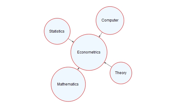
FIGURE 1.1: Interdisciplinarity of econometrics
\(~~~\)
Econometrics is interdisciplinary because it integrates economics, statistics, mathematics, and computer science to analyze economic data (FIGURE 1.1)
Population parameters \(\beta_0\) (constant term) and \(\beta_1\) (slope coefficient) are unknown as well as the error term \(u\), and they need to be estimated using observed variables \(x\) and \(y\)
Observed variables are typically associated with multiple cross-sectional units (such as households, individuals, cities, countries, \(\dots\)) at a given point in time, and therefore we use subscript \(i\) in the notation of these variables
There is a finite number of cross-sectional units \(i=1,2,3,...,n\), and thus EQUATION (1.2) holds for every observation
\[\begin{equation}\begin{matrix} y_1=\beta_0+\beta_1x_1+u_1 \\ y_2=\beta_0+\beta_1x_2+u_2 \\ \vdots \\ y_n=\beta_0+\beta_1x_n+u_n\end{matrix} \tag{1.3} \end{equation}\]
- A system of \(n\) equations (1.3) with two unknowns can be presented in matrix form
\[\begin{equation}\begin{bmatrix} y_1 \\ y_2 \\ \vdots \\ y_n\end{bmatrix}=\begin{bmatrix} 1 & x_1 \\ 1 & x_2 \\ \vdots & \vdots \\ 1 & x_n\end{bmatrix}\begin{bmatrix} \beta_0 \\ \beta_1 \end{bmatrix}+\begin{bmatrix} u_1 \\ u_2 \\ \vdots \\u_n\end{bmatrix} \tag{1.4} \end{equation}\]
The matrix equation \[\begin{equation} y=x\beta+u \tag{1.5} \end{equation}\] describes population regression model
- Data are usually presented as matrices and/or vectors, which simplifies computational operations in the background of any applied method.