4.1 RStudio – part A

There is also a cloud version of RStudio called Posit Cloud, which allows users to run RStudio in a web browser without needing to install anything locally
In 2022, RStudio rebranded as Posit, reflecting its expansion and integration with Python
RStudio cloud version is also free and available on this link https://posit.cloud/
The easiest way to access Posit Cloud is to log in with Google account (even if you are a first time user)
After running RStudio (on your PC or web browser) the user interface will look similar to the next screen
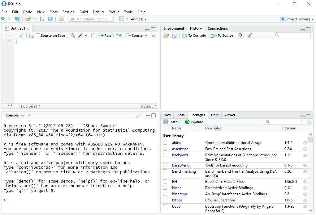
FIGURE 4.1: RStudio user interface
Unnamed file in the upper right corner Untitled1 is newly opened and empty R Script in which you write commands by hand (File -> New File -> R Script)
Arguments for each command are written inside the round brackets or parentheses ( )
Command is computed by selecting it with the mouse and clicking the Run button or by using the shortcut Ctrl+Enter at the end of the command line
It is useful to write a comments (lines beginning with
#) which are ignored by R. Comments are useful for making short notes in explaining your codes.In the lower left corner a Console window prints the results as well as warnings and errors (for example, the syntax of the command is incorrectly written or the specific command/object is not found)
Right side window panes serve to track the steps of the analysis, including History, Plots, Help, Packages (shows the list of currently installed packages in the library), etc.
Solution
Copy the code lines below to the clipboard and paste them into an R Script file opened in RStudio. Select each line separately (or all lines together) with the mouse and click theRun button. The results will be displayed in the Console window (bottom-left pane of RStudio). Any line starting with # is a comment, not a command. RStudio ignores comments by not running them.
# Some simple calculations
8*3
pi/2
exp(3)
sqrt(4)
5+4
log(10)
6^2
\(~~\)
a. Create a histogram of the same object a. Use fixed starting point of RNG (Random Number Generator).
Solution
Copy the code lines below to the clipboard and paste them into an R Script file opened in RStudio. Highlight each line separately (or all lines together) with the mouse, then click theRun button or press the Ctr + Enter shortcut). The object a will appear as a numerical array in the workspace Environment (top-right pane), and histogram will be displayed in the Plots pane (bottom-right).
# Generating random numbers and plotting them by histogram
set.seed(123)
a=rnorm(1000,0,1)
hist(a,main="Histogram of generated random numbers")
\(~~\)
First command
set.seed()is useful for creating reproducible random numbers (if omitted random numbers would differ every time you run the command in the second line)In the second line
rnorm()command generates random numbers from a normal distribution, and these numbers are assigned to object (variable)a. This allows you to reuse the generated random numbers later in your code. Instead of=assignment operator<-also can be used.The
hist()command creates a histogram of the data, while argumentmainis used to set the title of the histogram within quotes" ".
a again by a histogram but with a relative frequencies (probabilities), and add a normal curve to the same histogram.
Solution
Copy the code lines below to the clipboard, paste them into an R Script file opened in RStudio, and run them. A new histogram with a normal curve will appear in the Plots pane (bottom-right).# Adding a normal curve with red color to the histogram
hist(a,prob=TRUE,main="Histogram with a normal curve",xlab="generated random numbers")
curve(dnorm(x,0,1),col="red",add=TRUE)\(~~~\)
- It is possible to combine more commands in a single line, i.e.
dnorm()command is used insidecurve()command.
a. Provide statistical summary of the same object including minimum, maximum, median, mean, and quartiles.
Solution
Copy the code lines below to the clipboard, paste them into an R Script file opened in RStudio, and run them. The results will be displayed in the Console window (bottom-left pane of RStudio). Note: if some data are missing themean() and sd() commands will return a result only if the missing values are removed beforehand by setting the logical argument na.rm=TRUE inside parentheses of the same commands.
# Mean, standard deviation and statistical summary
mean(a)
sd(a)
summary(a)
\(~~~\)
- To summarize the results in well-formatted and customizable tables an additional package
modelsummaryshould be installed and loaded from the library. This package supportsdatasummary()command to visualize descriptive statistics andmodelsummary()command to visualize econometric model output.
modelsummary, use command datasummary() to present the mean and standard deviation of on object a in a well-formatted table. Convert numeric object a into data frame named dt.
Solution
Copy the code lines below to the clipboard, paste them into an R Script file opened in RStudio, and run them. A data frame objectdt will appear in the workspace Environment, and a table containing fundamental statistics will be displayed in the Viewer pane (bottom-right).
# Statistical summary by datasummary() command
install.packages("modelsummary")
library(modelsummary)
dt=data.frame(a)
datasummary(a~min+max+mean+sd,data=dt,fmt=4)
\(~~~\)
New object
dtis a data frame with one column. Commanddatasummary()requires data to be of typedata frame. Data frame, in general, may contain multiple columns of different types (numeric, character, factor or integer). Rows and columns of any data frame can be named/renamed, which helps in referencing to specific data in later usage.Once installed, packages do not need to be reinstalled, but they must be loaded from the library each time you use them in a new session.
The first argument of command
datasummary()is two-sidedformulawhich uses~symbol, while last argumentfmtcontrols the number of digits.
TABLE 3.1, assign life expectancy to variable y and poverty rate to variable x by hand. Create a scatter plot of these two variables. Merge both variables into another data frame called mydata. Rename the columns of mydata object as life and poverty. Assign countries names to the rows. Report descriptive statistics of both variables in a single table using command datasummary().
Solution
Copy the code lines below to the clipboard, paste them into an R Script file opened in RStudio, and run them. Variablesy and x are created by the c() function, which allows you to manually input data inside parentheses, separated by commas. Both variables will appear as numeric arrays in the workspace Environment, and a scatter plot will be displayed in the Plots pane. Data frame mydata will also appear in the workspace Envorinent, and finally a table containing fundamental statistics with respect to life and poverty will be displayed in the Viewer pane.
# Inputing data by hand as variables y and x
y=c(71.4,77.2,77.2,76.7,82.7,73.1,74.3,75.5,72.8,80.7)
x=c(31.7,10.7,22.2,20.9,25.2,26.1,19.4,16.8,34.4,13.2)
# Creating scatter plot with blue solid points and labeling the x-axis and y-axis
plot(x,y,main="Scatter plot",xlab="poverty rate",ylab="life expectancy",pch=19,col="blue")
# Merging both variables into another data frame with named columns and rows
mydata=data.frame(y,x)
colnames(mydata)=c("life","poverty")
rownames(mydata)=c("Bulgaria","Czech","Estonia","Croatia","Italy","Latvia","Hungary","Poland","Romania","Slovenia")
# Descriptive statistics of both variables
datasummary(life+poverty~min+max+mean+sd,data=mydata,fmt=4)
\(~~~\)
Save the R script with an arbitrary name of your choice (File -> Save as \(\dots\))
You can load a saved script into RStudio at any time, and the commands in that script will be recomputed by selecting them again and clicking the Run button
According to the RStudio settings, all scripts (with extension .R) are saved in your working directory; usually My Documents or Desktop
getwd() # Information about your current working directory
setwd("new path") # Working directory can be changed by setting a new path