9.1 Impulse response function
- IRF for ARDL\((1,0)\) is given as
\[\begin{equation} IRF=\left\{\begin{array}{cl} 0 & for~t=0~(period~zero)\\\beta_1 \beta_3^{t-1} & for~t=1,2,...,\infty~(all~future~periods)\end{array}\right. \tag{9.8} \end{equation}\]
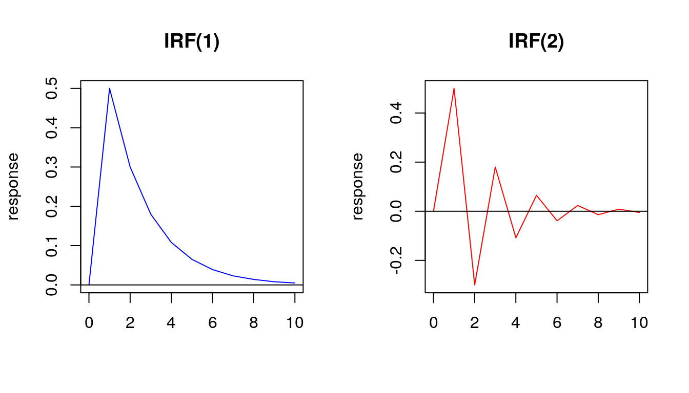
- The impulse response function IRF of the partial adjustment model ARDL\((1,0)\) can be represented in the table and on the figure
| Period | Response |
|---|---|
| \(~~~~~~~0~~~~~~~\) | \(0\) |
| \(1\) | \(\beta_1\) |
| \(2\) | \(\beta_1 \beta_3\) |
| \(3\) | \(\beta_1 \beta_3^2\) |
| \(4\) | \(\beta_1 \beta_3^3\) |
| \(5\) | \(\beta_1 \beta_3^4\) |
| \(\cdots\) | \(~~~~~~~~~~\cdots~~~~~~~~~~\) |
- The sum of the responses in all future periods represents the long-term effect of the variable \(x_t\) on the variable \(y_t\), i.e. the sum of the geometric series converges to
\[\begin{equation} \sum_{t=1}^\infty \beta_1 \beta_3^{t-1}=\frac{\beta_1}{1-\beta_3} \tag{9.9} \end{equation}\]
- Let’s consider following two examples
\[~~~~y_t=2+0.5x_t+0.6y_{t-1}+u_t~~~~~~~~~~~~~~~~~~~~~~~y_t=2+0.5x_t-0.6y_{t-1}+u_t\]

The impacts of the variable \(x_t\) on the variable \(y_t\) decline geometrically under the condition that \(|\beta_3|<1\), which means that the rate at which these impacts decay depends on the value of the parameter \(\beta_3\)
The sign of the parameter \(\beta_3\) influences the shape of the impulse response function
In the long-run, the variables are expected to be in equilibrium or steady state
The long-run equilibrium equation of the partial adjustment model ARDL\((1,0)\) is
\[\begin{equation} y^E=\frac{\beta_0}{1-\beta_3}+\frac{\beta_1}{1-\beta_3}x^E \tag{9.10} \end{equation}\]
Exercise 39. Based on the partial adjustment model ARDL\((1,0)\)
\[y_t=2+0.5x_t+0.6y_{t-1}+u_t\]
determine:
- Short-run effect of \(x_t\) on \(y_t\)
- Long-run effect of \(x_t\) on \(y_t\)
- Speed of decreasing responses
- Equilibrium equation
Solution
Short-run effect is \(0.5\) (the response in the first period \(\beta_1=0.5\)). Long-run effect is \(1.25\) computed by formula \(\frac{\beta_1}{1-\beta_3}=\frac{0.5}{1-0.6}=1.25\). Responses in each period are decreasing at speed rate of \(40\%\) according to \((\beta_3-1)100\%=(0.6-1)100\%=-40\%\). Equilibrium equation is \(y^E=5+1.25x^E\).- IRF for a ARDL\((1,1)\) is given as
\[\begin{equation} IRF=\left\{\begin{array}{cl} 0 & for~t=0~(period~zero)\\ \beta_1 & for~t=1~(first~period)\\ (\beta_2+ \beta_1\beta_3)\beta_3^{t-1} & for~t=2,3,...,\infty~(all~future~periods)\end{array}\right. \tag{9.11} \end{equation}\]
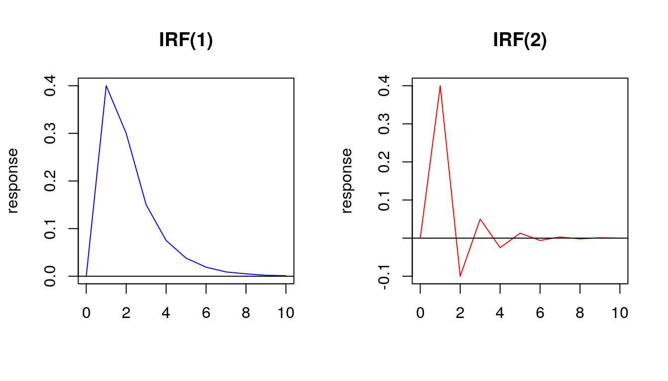
- The impulse response function IRF of the ARDL\((1,1)\) can also be represented in the table and on the figure
| Period | Response |
|---|---|
| \(~~~~~~~0~~~~~~~\) | \(0\) |
| \(1\) | \(\beta_1\) |
| \(2\) | \(\beta_2+\beta_1 \beta_3\) |
| \(3\) | \((\beta_2+\beta_1 \beta_3)\beta_3\) |
| \(4\) | \((\beta_2+\beta_1 \beta_3)\beta_3^2\) |
| \(5\) | \((\beta_2+\beta_1 \beta_3)\beta_3^3\) |
| \(\cdots\) | \(~~~~~~~~~~\cdots~~~~~~~~~~\) |
- Likewise, the sum of responses in all future periods represents the long-term effect of the variable \(x_t\) on the variable \(y_t\)
\[\begin{equation} \sum_{t=1}^\infty \frac{\Delta y_{T+t}}{\Delta x_t}=\frac{\beta_1+\beta_2}{1-\beta_3} \tag{9.12} \end{equation}\]
- Let’s consider two additional examples
\[y_t=7+0.4x_t+0.1x_{t-1}+0.5y_{t-1}+u_t~~~~~~~~~~~~~~~~~~~~~~~y_t=7+0.4x_t+0.1x_{t-1}-0.5y_{t-1}+u_t\]

- Equilibrium or long-run equation based on ARDL\((1,1)\) is
\[\begin{equation} y^E=\frac{\beta_0}{1-\beta_3}+\frac{\beta_1+\beta_2}{1-\beta_3}x^E \tag{9.13} \end{equation}\]
Equilibrium state may exist only if variables are related in the long-run
If variables are related in the long-run then they are related in the short-run also (not necessary conversely)
If variables are related both in the short-run and in the long-run it is evidence of cointegration
Exercise 40. Using model ARDL\((1,1)\)
\[y_t=5+0.3x_t+0.2x_{t-1}+0.7y_{t-1}+u_t\]
determine:
- Short-run effect of \(x_t\) on \(y_t\)
- Long-run effect of \(x_t\) on \(y_t\)
- Speed of decreasing responses
- Equilibrium equation
Solution
Short-run effect is \(0.3\) (the response in the first period \(\beta_1=0.3\)). Long-run effect is \(1.67\) computed by formula \(\frac{\beta_1+\beta_2}{1-\beta_3}=\frac{0.3+0.2}{1-0.7}=1.67\). Responses in each period are decreasing at speed rate of \(30\%\) according to \((\beta_3-1)100\%=(0.7-1)100\%=-30\%\). Equilibrium equation is \(y^E=16.67+1.67x^E\).indicators estimate three models: ARDL\((0,0)\), ARDL\((1,0)\) and ARDL\((1,1)\) with names static, dynamic1 and dynamic2, respectively. For that purpose apply dynlm() commad from the package dynlm, assuming that variable \(x_t\) is production and variable \(y_t\) is growth. Present the results of estimated models in a single table by modelsummary() command. Which model fits the data better? For all three models check if the first-order autocorrleation problem exist by employing bgtest() command from the package lmtest. Based on partial adjustment model calculate the short-run and the long-run effect of the production on the growth rate.
Solution
In this example an evidence of autocorrelation problem in static model is found according to Breusch-Godfrey test of order up to \(1\). Opposite to that, both dynamic modelsdynamic1 and dynamic2 do not exhibit autocorrelation problem as it is absorbed by including lagged growth on the RHS \((y_{t-1})\). Note that within dynlm() command a lagged variable is computed using a lag operator L(). Partial adjustment model dynamic1 fits the data better in terms of \(R^2\) and statistical significance of the estimated parameters. According to that model a short-run effect of production to the growth rate is \(0.166\%\), and the long-run effect is \(0.574\%\) (both effects are expressed in \(\%\) as both variable \(x_t\) and \(y_t\) are given in percentages).
# Installing and loading dynlm package
install.packages("dynlm")
library(dynlm)

# Estimating three model by applying dynlm() command
static=dynlm(growth~production,data=indicators)
dynamic1=dynlm(growth~production+L(growth),data=indicators)
dynamic2=dynlm(growth~production+L(production)+L(growth),data=indicators)

# Presenting results in a single table
library(modelsummary) # loading the package modelsummary (if you are runing a new session)
modelsummary(list(static,dynamic1,dynamic2),stars=TRUE,fmt=4)

library(lmtest) # loading the package lmtest (if you are runing a new session)
bgtest(static)
bgtest(dynamic1)
bgtest(dynamic2)

# Short-run effect is the second coefficient from "dynamic1" model
coef(dynamic1)[2]

# Long-run effect is the ratio between the second coefficient and 1 minus the third coefficient from "dynamic1" model
coef(dynamic1)[2]/(1-coef(dynamic1)[3])
\(~~~\)