4.3 Worked Example

Helene Wagner

1. Overview of Worked Example

a. Goals

This worked example shows:

How microsatellite data may be coded in a spreadsheet.
How such a file is imported into R.
How the data are imported into a ‘genind’ object using package ‘adegenet’.
How to view information stored in a ‘genind’ object.
How to import the data with the ‘gstudio’ package.
How to import SNP data

Try modifying the code to import your own data!

b. Data set

This code imports genetic data from 181 individuals of Colombia spotted frogs (Rana luteiventris) from 12 populations. The data are a subsample of the full data set analyzed in Funk et al. (2005) and Murphy et al. (2010). Please see the separate introduction to the data set.

ralu.loci: Data frame with populations and genetic data (181 rows x 9 columns). Included in package LandGenCourse.

c. Required R packages

Install some packages needed for this worked example. Note: popgraph needs to be installed before installing gstudio.

if(!require("adegenet")) install.packages("adegenet")
if(!requireNamespace("popgraph", quietly = TRUE))
{
  install.packages(c("RgoogleMaps", "geosphere", "proto", "sampling", 
                      "seqinr", "spacetime", "spdep"), dependencies=TRUE)
  remotes::install_github("dyerlab/popgraph")
}
if(!requireNamespace("gstudio", quietly = TRUE)) remotes::install_github("dyerlab/gstudio")

## Warning: replacing previous import 'dplyr::union' by 'raster::union' when
## loading 'gstudio'

## Warning: replacing previous import 'dplyr::intersect' by 'raster::intersect'
## when loading 'gstudio'

## Warning: replacing previous import 'dplyr::select' by 'raster::select' when
## loading 'gstudio'

Note: the function library will always load the package, even if it is already loaded, whereas require will only load it if it is not yet loaded. Either will work.

library(adegenet)
library(gstudio)
library(LandGenCourse)
library(tibble)
library(here)
library(vcfR)
library(pinfsc50)
library(utils)

2. Import data from .csv file

a. Preparation

Create a new R project for this lab: File > New Project > New Directory > New Project.

This will automatically set your working directory to the new project folder. That’s where R will look for files and save anything you export.

Note: R does not distinguish between single quotes and double quotes, they are treated as synonyms, but the opening and closing symbols need to match.

The dataset ralu.loci is available in the package ‘LandGenCourse’ and can be loaded with data(ralu.loci).

data(ralu.loci)

Below, however, we’ll import it from a comma separated file (.csv), as this is the recommended format for importing your own data (e.g. from Excel).

b. Excel file

First we need to copy the file ralu.loci.csv to the downloads folder inside your project folder. The first line checks that the folder downloads exists and creates it if needed.

if(!dir.exists(paste0(here(),"/downloads"))) dir.create(paste0(here(),"/downloads"))
file.copy(system.file("extdata", "ralu.loci.csv", package = "LandGenCourse"),
          paste0(here(), "/downloads/ralu.loci.csv"), overwrite=FALSE)

## [1] FALSE

Check that the file ralu.loci.csv is now in the folder downloads within your project folder. From your file system, you can open it with Excel. Note that in Excel, the columns with the loci must be explicitly defined as ‘text’, otherwise Excel is likely to interpret them as times.

Excel instructions:

Opening an existing .csv file with genetic data:

Excel menu: ‘File > New Workbook’.
Excel menu: ‘File > Import > CSV File > Import’. Navigate to file.
Text Import Wizard: select ‘Delimited’, click ‘Next’.
Delimiters: check ‘comma’. Click ‘Next’.
Use the ‘Shift’ key to select all columns with loci A - H. Select ‘text’. Click ‘Finish > OK’.

Creating a new Excel file to enter genetic data:

Label the loci columns.
Select all loci columns by clicking on the column headers (hold the ‘Shift’ key to select multiple adjacent columns).
Define the data format: ‘Format > Cell > Text’.
Enter genetic data, separating the alleles by a colon (e.g., ‘1:3’).

Saving Excel file for import in R:

File Format: ‘Comma Separated Values (.csv)’

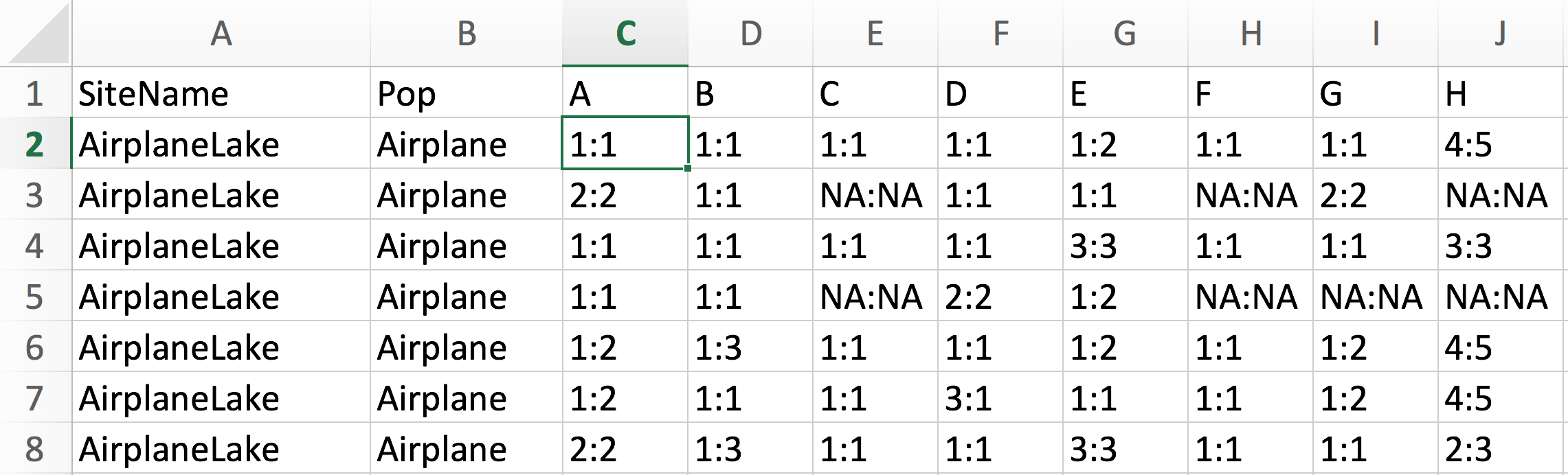
Here is a screenshot of the first few lines of the Excel file with the genetic data:

c. Import with function ‘read.csv’

As the file is saved in csv format, we use the function ‘read.csv’ to import it into an R object called Frogs. Display the first few rows and columns to check whether the data have been imported correctly:

Frogs <- read.csv(paste0(here(), "/downloads/ralu.loci.csv"), header=TRUE)
as_tibble(Frogs)

## # A tibble: 181 × 10
##    SiteName     Pop      A     B     C     D     E     F     G     H    
##    <chr>        <chr>    <chr> <chr> <chr> <chr> <chr> <chr> <chr> <chr>
##  1 AirplaneLake Airplane 1:1   1:1   1:1   1:1   1:2   1:1   1:1   4:5  
##  2 AirplaneLake Airplane 2:2   1:1   NA:NA 1:1   1:1   NA:NA 2:2   NA:NA
##  3 AirplaneLake Airplane 1:1   1:1   1:1   1:1   3:3   1:1   1:1   3:3  
##  4 AirplaneLake Airplane 1:1   1:1   NA:NA 2:2   1:2   NA:NA NA:NA NA:NA
##  5 AirplaneLake Airplane 1:2   1:3   1:1   1:1   1:2   1:1   1:2   4:5  
##  6 AirplaneLake Airplane 1:2   1:1   1:1   3:1   1:1   1:1   1:2   4:5  
##  7 AirplaneLake Airplane 2:2   1:3   1:1   1:1   3:3   1:1   1:1   2:3  
##  8 AirplaneLake Airplane 2:2   1:3   1:1   1:1   3:3   1:1   1:1   2:3  
##  9 AirplaneLake Airplane 3:1   1:1   1:1   1:1   1:7   1:1   1:1   3:5  
## 10 AirplaneLake Airplane 2:2   1:3   1:1   1:1   3:7   1:1   1:1   3:3  
## # ℹ 171 more rows

The data frame Frogs contains 181 rows and 11 columns. Only the first few are shown.
The file has a header row with column names.
Notice the abbreviations for the R data type under each variable name: <fctr> means that the variable has been coded as a factor.
Each row is one individual. Note that for this data set, there is no column with ID or names of individuals.
The first two columns indicates the site in long (“SiteName”) and short (“Pop”) format.
There are 8 columns with loci, named A - H. Each locus has two alleles, coded with numbers and separated by a colon (:).
This coding suggests that the markers are codominant and that the species is diploid.
The code for missing values is NA, (which shows up as NA:NA for missing genetic data). There seem to be quite a few missing values.

d. Create ID variable

We’ll add unique ID’s for the frogs (to show how these would be imported). Here we take, for each frog, a sub-string of Pop containing the first three letters, add the row number, and separate them by a period.

Frogs <- data.frame(FrogID = paste(substr(Frogs$Pop, 1, 3), row.names(Frogs), sep="."), Frogs)
as_tibble(Frogs)

## # A tibble: 181 × 11
##    FrogID SiteName     Pop      A     B     C     D     E     F     G     H    
##    <chr>  <chr>        <chr>    <chr> <chr> <chr> <chr> <chr> <chr> <chr> <chr>
##  1 Air.1  AirplaneLake Airplane 1:1   1:1   1:1   1:1   1:2   1:1   1:1   4:5  
##  2 Air.2  AirplaneLake Airplane 2:2   1:1   NA:NA 1:1   1:1   NA:NA 2:2   NA:NA
##  3 Air.3  AirplaneLake Airplane 1:1   1:1   1:1   1:1   3:3   1:1   1:1   3:3  
##  4 Air.4  AirplaneLake Airplane 1:1   1:1   NA:NA 2:2   1:2   NA:NA NA:NA NA:NA
##  5 Air.5  AirplaneLake Airplane 1:2   1:3   1:1   1:1   1:2   1:1   1:2   4:5  
##  6 Air.6  AirplaneLake Airplane 1:2   1:1   1:1   3:1   1:1   1:1   1:2   4:5  
##  7 Air.7  AirplaneLake Airplane 2:2   1:3   1:1   1:1   3:3   1:1   1:1   2:3  
##  8 Air.8  AirplaneLake Airplane 2:2   1:3   1:1   1:1   3:3   1:1   1:1   2:3  
##  9 Air.9  AirplaneLake Airplane 3:1   1:1   1:1   1:1   1:7   1:1   1:1   3:5  
## 10 Air.10 AirplaneLake Airplane 2:2   1:3   1:1   1:1   3:7   1:1   1:1   3:3  
## # ℹ 171 more rows

e. Export with function ‘write.csv’

If you want to export (and import) your own files, adapt this code.

Note: when using R Notebooks, problems can arise if R looks for files in a different place (more on this in Week 8 Bonus material). Here, we use a safe work-around, with the function here, that will help make your work reproducible and transferable to other computers. For this to work properly, you must work within an R project, and you must have writing permission for the project folder.

The function here from the package here finds the path to your project folder. Remove the hashtags and run the two lines to see the path to your project folder, and the path to the (to be created) output folder. The function paste0 simply pastes strings of text together, without any separator (hence the ‘0’ in the function name).

here()

## [1] "/Users/helene/Desktop/R_Github_projects/LandGenCourse_book"

paste0(here(),"/output")

## [1] "/Users/helene/Desktop/R_Github_projects/LandGenCourse_book/output"

The following line checks whether an output folder exists in the project folder, and if not, creates one.

if(!dir.exists(paste0(here(),"/output"))) dir.create(paste0(here(),"/output"))

Now we can write our data into a csv file in the output folder:

write.csv(ralu.loci, paste0(here(),"/output/ralu.loci.csv"), 
          quote=FALSE, row.names=FALSE)

To import the file again from the output folder, you could do this:

ralu.loci.2 <- read.csv(paste0(here(),"/output/ralu.loci.csv"), header=TRUE)

3. Create ‘genind’ Object

a. Read the helpfile

We use the function df2genind of the adegenet package to import the loci into a genind object named Frogs.genind. Check the help file for a definition of all arguments and for example code.

?df2genind

b. Set all arguments of function ‘df2genind’

Some explanations:

X: this is the data frame (or matrix) containing the loci only. Hence we need columns 4 - 11.
sep: need to specify the separator between alleles (here: colon)
ncode: not needed here because we used a separator, defined under sep.
ind.names: here we should indicate the column FrogID.
loc.names: by default this will use the column names of the loci.
pop: here we should indicate either the column Pop or SiteName.
NA.char: how were missing values coded? Here: NA.
ploidy: this species is diploid, hence 2.
type: marker type, either "codom" for codominant markers like microsatellites, or "PA" for presence-absence, such as SNP or AFLP markers. Note: you can use either “” or ’’.
strata: one way of defining hierarchical sampling levels. We will add this in Week 3.
hierarchy: another way of defining hierarchical sampling levels. We’ll skip it for now.

Frogs.genind <- df2genind(X=Frogs[,c(4:11)], sep=":", ncode=NULL, ind.names= Frogs$FrogID, loc.names=NULL, pop=Frogs$Pop, NA.char="NA", ploidy=2, type="codom", strata=NULL, hierarchy=NULL)

c. Check imported data

Printing the genind object’s name lists the number of individuals, loci and alleles, and lists all slots (prefaced by @).

Frogs.genind

## /// GENIND OBJECT /////////
## 
##  // 181 individuals; 8 loci; 39 alleles; size: 55.2 Kb
## 
##  // Basic content
##    @tab:  181 x 39 matrix of allele counts
##    @loc.n.all: number of alleles per locus (range: 3-9)
##    @loc.fac: locus factor for the 39 columns of @tab
##    @all.names: list of allele names for each locus
##    @ploidy: ploidy of each individual  (range: 2-2)
##    @type:  codom
##    @call: df2genind(X = Frogs[, c(4:11)], sep = ":", ncode = NULL, ind.names = Frogs$FrogID, 
##     loc.names = NULL, pop = Frogs$Pop, NA.char = "NA", ploidy = 2, 
##     type = "codom", strata = NULL, hierarchy = NULL)
## 
##  // Optional content
##    @pop: population of each individual (group size range: 7-23)

d. Summarize ‘genind’ object

There is a summary function for genind objects. Notes:

Group here refers to the populations, i.e., Group sizes means number of individuals per population.
It is a good idea to check the percentage of missing values here. If it is 0%, this may indicate that the coding for missing values was not recognized. If the % missing is very high, on the other hand, there may be some other importing problem.

summary(Frogs.genind)

## 
## // Number of individuals: 181
## // Group sizes: 21 8 14 13 7 17 9 20 19 13 17 23
## // Number of alleles per locus: 3 4 4 4 9 3 4 8
## // Number of alleles per group: 21 21 20 22 20 19 19 25 18 14 18 26
## // Percentage of missing data: 10.64 %
## // Observed heterozygosity: 0.1 0.4 0.09 0.36 0.68 0.02 0.38 0.68
## // Expected heterozygosity: 0.17 0.47 0.14 0.59 0.78 0.02 0.48 0.74

4. View information stored in ‘genind’ object

The summary lists each attribute or slot of the genind object and summarizes its content. Technically speaking, genind objects are S4 objects in R, which means that their slots are accessed with the @ sign, rather than the $ sign for attributes of the more commonly used S3 objects. Interestingly, the object does not store the data table that was imported, but converts it to a table of allele counts.

a. Slot `@tab`

Table with allele counts, where each column is an allele. Allele name A.1 means “locus A, allele 1”. For a codominant marker (e.g. microsatellite) and a diploid species, allele counts per individual can be 0, 1, 2, or NA=missing. Here are the first few lines:

as_tibble(Frogs.genind@tab)

## # A tibble: 181 × 39
##      A.1   A.2   A.3   B.1   B.3   B.2   B.4   C.1   C.2   C.4   C.5   D.1   D.2
##    <int> <int> <int> <int> <int> <int> <int> <int> <int> <int> <int> <int> <int>
##  1     2     0     0     2     0     0     0     2     0     0     0     2     0
##  2     0     2     0     2     0     0     0    NA    NA    NA    NA     2     0
##  3     2     0     0     2     0     0     0     2     0     0     0     2     0
##  4     2     0     0     2     0     0     0    NA    NA    NA    NA     0     2
##  5     1     1     0     1     1     0     0     2     0     0     0     2     0
##  6     1     1     0     2     0     0     0     2     0     0     0     1     0
##  7     0     2     0     1     1     0     0     2     0     0     0     2     0
##  8     0     2     0     1     1     0     0     2     0     0     0     2     0
##  9     1     0     1     2     0     0     0     2     0     0     0     2     0
## 10     0     2     0     1     1     0     0     2     0     0     0     2     0
## # ℹ 171 more rows
## # ℹ 26 more variables: D.3 <int>, D.4 <int>, E.1 <int>, E.2 <int>, E.3 <int>,
## #   E.7 <int>, E.6 <int>, E.8 <int>, E.5 <int>, E.4 <int>, E.10 <int>,
## #   F.1 <int>, F.2 <int>, F.3 <int>, G.1 <int>, G.2 <int>, G.3 <int>,
## #   G.5 <int>, H.4 <int>, H.5 <int>, H.3 <int>, H.2 <int>, H.1 <int>,
## #   H.6 <int>, H.8 <int>, H.7 <int>

b. Slot `@loc.n.all`

Number of alleles per locus, across all populations.

Frogs.genind@loc.n.all

## A B C D E F G H 
## 3 4 4 4 9 3 4 8

c. Slot `@loc.fac`

This is a factor that indicates for each allele (column in @tab) which locus it belongs to. The levels of the factor correspond to the loci.

Frogs.genind@loc.fac

##  [1] A A A B B B B C C C C D D D D E E E E E E E E E F F F G G G G H H H H H H H
## [39] H
## Levels: A B C D E F G H

d. Slot `@all.names`

List of allele names, separately for each locus. Note: the alleles are treated as text (character), even if they are coded as numbers. They are sorted in order of occurrence in data set.

Frogs.genind@all.names

## $A
## [1] "1" "2" "3"
## 
## $B
## [1] "1" "3" "2" "4"
## 
## $C
## [1] "1" "2" "4" "5"
## 
## $D
## [1] "1" "2" "3" "4"
## 
## $E
## [1] "1"  "2"  "3"  "7"  "6"  "8"  "5"  "4"  "10"
## 
## $F
## [1] "1" "2" "3"
## 
## $G
## [1] "1" "2" "3" "5"
## 
## $H
## [1] "4" "5" "3" "2" "1" "6" "8" "7"

e. Further slots

The following slots are automatically filled with default values unless specified by user during import into genind object:

Slot @ploidy: ploidy for each individual.
Slot @type: codominant (microsatellites) or presence/absence (SNP, AFLP)

The following slots may be empty unless specified during or after import into ‘genind’ object:

Slot @other: placeholder for non-genetic data, e.g. spatial coordinates of individuals.
Slot @pop: vector indicating the population that each individual belongs to.
Slot @strata: stratification of populations, e.g. within regions or treatments.
Slot @hierarchy: optional formula defining hierarchical levels in strata.

5. Import data with ‘gstudio’ package

a. Function ‘read_population’

While genind objects are used by many functions for analyzing genetic data, the gstudio package provides an interface for additional analysis. We use the function read_population to import the data.

?read_population

b. Set arguments

Some explanations:

path: This is the path to the .csv file. If it is in the current working directory, then the filename is sufficient.
type: here we have ‘separated’ data, as the alleles at each locus are separated by a colon.
locus.columns: this would be columns 3 - 10 in this case, because we are importing from the .csv file directly, which does not contain the FrogID variable. We can add that later.
phased: default is fine here.
sep: here this refers to the .csv file! The separater is a comma.
header: yes we have column names.

Working directory confusion: If you are working within an R project folder, then that folder is automatically set as your working directory. If you are working in an R session outside of an R project, then you need to actively set the working directory in the R Studio menu under: Session > Set working directory > Choose Directory.

Frogs.gstudio <- read_population(path=system.file("extdata", "ralu.loci.csv", 
                                                  package = "LandGenCourse"), 
                   type="separated", locus.columns=c(3:10), 
                   phased=FALSE, sep=",", header=TRUE)

c. Check imported data

Check the column types: SiteName and Pop are now character vectors, and the loci columns A - H are now of class locus (it is indicated that ‘locus’ is a S3 object type).

str(Frogs.gstudio)

## 'data.frame':    181 obs. of  10 variables:
##  $ SiteName: chr  "AirplaneLake" "AirplaneLake" "AirplaneLake" "AirplaneLake" ...
##  $ Pop     : chr  "Airplane" "Airplane" "Airplane" "Airplane" ...
##  $ A       : 'locus' chr  "1:1" "2:2" "1:1" "1:1" ...
##  $ B       : 'locus' chr  "1:1" "1:1" "1:1" "1:1" ...
##  $ C       : 'locus' chr  "1:1" "" "1:1" "" ...
##  $ D       : 'locus' chr  "1:1" "1:1" "1:1" "2:2" ...
##  $ E       : 'locus' chr  "1:2" "1:1" "3:3" "1:2" ...
##  $ F       : 'locus' chr  "1:1" "" "1:1" "" ...
##  $ G       : 'locus' chr  "1:1" "2:2" "1:1" "" ...
##  $ H       : 'locus' chr  "4:5" "" "3:3" "" ...

d. Add FrogID

Frogs.gstudio is a data frame, and we can manipulate like any other data frame. Here we will add the variable FrogID as the first column.

Frogs.gstudio <- data.frame(FrogID=Frogs$FrogID, Frogs.gstudio) 
head(Frogs.gstudio)

##   FrogID     SiteName      Pop   A   B   C   D   E   F   G   H
## 1  Air.1 AirplaneLake Airplane 1:1 1:1 1:1 1:1 1:2 1:1 1:1 4:5
## 2  Air.2 AirplaneLake Airplane 2:2 1:1     1:1 1:1     2:2    
## 3  Air.3 AirplaneLake Airplane 1:1 1:1 1:1 1:1 3:3 1:1 1:1 3:3
## 4  Air.4 AirplaneLake Airplane 1:1 1:1     2:2 1:2            
## 5  Air.5 AirplaneLake Airplane 1:2 1:3 1:1 1:1 1:2 1:1 1:2 4:5
## 6  Air.6 AirplaneLake Airplane 1:2 1:1 1:1 1:3 1:1 1:1 1:2 4:5

e. Convert to ‘genind’ object

We can use the dataframe with the locus objects from gstudio to import the data into a genind object. In this case, we set sep=":", because the locus object in gstudio stores the alleles at each locus separated by a colon, and NA.char="", because gstudio stores missing values as empty cells.

Frogs.genind2 <- adegenet::df2genind(X=Frogs.gstudio[,c(4:11)], sep=":", ncode=NULL,   
                          ind.names=Frogs.gstudio$FrogID, loc.names=NULL, 
                          pop=Frogs.gstudio$Pop, NA.char="", ploidy=2, 
                          type="codom", strata=NULL, hierarchy=NULL)
Frogs.genind2

## /// GENIND OBJECT /////////
## 
##  // 181 individuals; 8 loci; 39 alleles; size: 55.5 Kb
## 
##  // Basic content
##    @tab:  181 x 39 matrix of allele counts
##    @loc.n.all: number of alleles per locus (range: 3-9)
##    @loc.fac: locus factor for the 39 columns of @tab
##    @all.names: list of allele names for each locus
##    @ploidy: ploidy of each individual  (range: 2-2)
##    @type:  codom
##    @call: adegenet::df2genind(X = Frogs.gstudio[, c(4:11)], sep = ":", 
##     ncode = NULL, ind.names = Frogs.gstudio$FrogID, loc.names = NULL, 
##     pop = Frogs.gstudio$Pop, NA.char = "", ploidy = 2, type = "codom", 
##     strata = NULL, hierarchy = NULL)
## 
##  // Optional content
##    @pop: population of each individual (group size range: 7-23)

6. Importing SNP data

a. Import from text file

First, we’ll import a relatively small SNP dataset from a text file. This dataset will be analyzed in the Week 6 Worked Example. The data are stored in a tab-delimited text file.

Let’s have a look at the first few rows and columns:

family: these are ID’s of the genotyped tree individuals (from which seeds were grown in a common-garden experiment, hence they are called “family” in the dataset).
population: the trees were sampled from a set of populations.
snpXXX.Plmn: each column is a diploid SNP.

To import your own data, replace infile by the path to the text file with your SNP data. Change settings as necessary (check whether data are separated by tabs or commas!).

infile <- system.file("extdata", "WWP_SNP_genotypes.txt", package = "LandGenCourse")
Trees <- read.table(infile, header = TRUE, sep = "\t")
Trees[1:6, 1:6]

##   family population snp102.Plmn snp106.Plmn snp108.Plmn snp110.Plmn
## 1     59    blk cyn          CC          AC          GG          GG
## 2     60    blk cyn          AC          AA          AG          GG
## 3     61    blk cyn          CC          AA          AG          GG
## 4     63    blk cyn          CC          AA          GG          GG
## 5     64    blk cyn          AC          AA          AG          GG
## 6     65    blk cyn          AC          AA        <NA>          GG

We should replace the SNP column names: if they contain a period ., then the function df2genind thinks that the first part indicates the locus and the second part the allele. The following line of code splits each column name by the period and only retains the first part.

names(Trees) <- unlist(lapply(names(Trees), function(x) strsplit(x, "[.]")[[1]][1]))

To import these data frame into a genind object, we need to tell R how the SNP data are coded (check the df2genind help file!)

ncode = 1: each allele (A, C, G, T) is coded with a single character.
sep = "": the two alleles per individual and locus are not separated by any symbol.
NA.char= "NA": missing values are coded as NA.

Trees.genind <- adegenet::df2genind(X=Trees[,-c(1:2)], sep="", ncode=1,   
                          ind.names=Trees$family, loc.names=NULL, 
                          pop=Trees$population, NA.char="NA", ploidy=2, 
                          type="codom", strata=NULL, hierarchy=NULL)
Trees.genind

## /// GENIND OBJECT /////////
## 
##  // 157 individuals; 164 loci; 324 alleles; size: 302 Kb
## 
##  // Basic content
##    @tab:  157 x 324 matrix of allele counts
##    @loc.n.all: number of alleles per locus (range: 1-2)
##    @loc.fac: locus factor for the 324 columns of @tab
##    @all.names: list of allele names for each locus
##    @ploidy: ploidy of each individual  (range: 2-2)
##    @type:  codom
##    @call: adegenet::df2genind(X = Trees[, -c(1:2)], sep = "", ncode = 1, 
##     ind.names = Trees$family, loc.names = NULL, pop = Trees$population, 
##     NA.char = "NA", ploidy = 2, type = "codom", strata = NULL, 
##     hierarchy = NULL)
## 
##  // Optional content
##    @pop: population of each individual (group size range: 9-22)

b. Import from vcf file to genind object

A common data format for genomic data is vcf. Here’s some background information (all but the first are vignettes from the vcfR package):

PDF defining the data format: https://samtools.github.io/hts-specs/VCFv4.3.pdf
Tutorial on data format: https://cran.r-project.org/web/packages/vcfR/vignettes/vcf_data.html
Tutorial on quality testing: https://cran.r-project.org/web/packages/vcfR/vignettes/intro_to_vcfR.html
Tutorial on converting vcf data: https://cran.r-project.org/web/packages/vcfR/vignettes/converting_data.html

The R package vcfR makes it easy to import vcf files and convert to other formats. Here we use it to convert the data into a genind object. The following code is adapted from the above listed vcfR vignettes.

We’ll import a file that is distributed with the pinfsc50 package. Note that vcf files are commonly compressed in gz archives. To import your own data, replace vcf_file by the path to your own gz archive.

vcf_file <- system.file("extdata", "pinf_sc50.vcf.gz", package = "pinfsc50")
vcf <- read.vcfR( vcf_file, verbose = FALSE )

Note that the package vcfR can import three types of genomic data files listed below. We will only use the .vcf file here.

.vcf: SNPs
.fasta: genomic reference sequence data
.gff: annotation

Convert to genind object:

SNP_genind <- vcfR2genind(vcf)
SNP_genind

## /// GENIND OBJECT /////////
## 
##  // 18 individuals; 22,031 loci; 44,137 alleles; size: 16.4 Mb
## 
##  // Basic content
##    @tab:  18 x 44137 matrix of allele counts
##    @loc.n.all: number of alleles per locus (range: 1-5)
##    @loc.fac: locus factor for the 44137 columns of @tab
##    @all.names: list of allele names for each locus
##    @ploidy: ploidy of each individual  (range: 2-2)
##    @type:  codom
##    @call: adegenet::df2genind(X = t(x), sep = sep)
## 
##  // Optional content
##    - empty -

c. Import from vcf file to genlight object

This dataset has 18 individuals genotyped at 44,137. It may be better to use a genlight object instead of genind. This is an alternative object type from the package adegenet that can store large genomic data much more efficiently.

Note: the current implementation can only store two alleles per locus, loci with more alleles will be dropped and a warning is printed.

SNP_genlight <- vcfR2genlight(vcf)

## Warning in vcfR2genlight(vcf): Found 312 loci with more than two alleles.
## Objects of class genlight only support loci with two alleles.
## 312 loci will be omitted from the genlight object.

SNP_genlight

##  /// GENLIGHT OBJECT /////////
## 
##  // 18 genotypes,  21,719 binary SNPs, size: 2.2 Mb
##  31239 (7.99 %) missing data
## 
##  // Basic content
##    @gen: list of 18 SNPbin
## 
##  // Optional content
##    @ind.names:  18 individual labels
##    @loc.names:  21719 locus labels
##    @chromosome: factor storing chromosomes of the SNPs
##    @position: integer storing positions of the SNPs
##    @other: a list containing: elements without names

Note that instead of 44,137 alleles, we now have 21,719 binary SNPs. This is one of the ways by which the genlight object is more efficient than genind. Overall, the size has been reduced from 16.4 Mb to 2.2 Mb!