Chapter 11 Lab 9 - Crimes, Times, and Places
Welcome to Lab 9! In this lab we are going to focus on:
Topics Covered
- Identifying patterns of person and property crime
- Linking times and places
- Thinking about crime tactically
11.1 Identifying Crimes and Places
Let’s start by reading in our data. We have three data files to work with today:
chicago_crime: A dataframe containing a large number of crimes in Chicago in 2019beat: A dataframe listing the location of over 134,000 crimes
One warning: Since there are so many incidents in the chicago_crime shapefile, it might take a minute or two to fully load into R. Just give it some time!
library(sf)
library(lubridate)
library(tidyverse)

chicago_crime <- st_read("C:/Users/gioc4/Desktop/chicago_crime.shp")
chicago_beat <- st_read("C:/Users/gioc4/Desktop/chicago_police_beat.shp")
11.1.1 Looking at crime types
First, we can examine the unique types of crime in ourchicago_crime dataframe. If you recall, we want to use the
functions glimpse to look at the variables, and summary or table to examine individual variables.
# Look at the names of the variables
glimpse(chicago_crime)
## Rows: 242,424
## Columns: 13
## $ id <dbl> 11947976, 11931877, 11897326, 11865011, 11861652, 11925609, 11922427, 11880462, 11769231, 11906880, 119053~
## $ crime <chr> "CRIMINAL SEXUAL ASSAULT", "BATTERY", "OFFENSE INVOLVING CHILDREN", "DECEPTIVE PRACTICE", "DECEPTIVE PRACT~
## $ crime_type <chr> "PREDATORY", "AGGRAVATED - HANDGUN", "AGGRAVATED CRIMINAL SEXUAL ABUSE BY FAMILY MEMBER", "COUNTERFEIT CHE~
## $ arrest <int> 0, 1, 1, 1, 1, 1, 0, 1, 0, 0, 0, 0, 1, 0, 1, 1, 1, 0, 1, 0, 1, 1, 0, 0, 0, 0, 0, 0, 0, 0, 0, 0, 1, 1, 0, 0~
## $ domestic <int> 1, 0, 1, 0, 0, 0, 0, 0, 0, 0, 0, 0, 0, 0, 0, 0, 0, 0, 0, 0, 0, 1, 0, 0, 0, 0, 0, 0, 0, 0, 0, 1, 0, 0, 0, 0~
## $ beat <chr> "0434", "0911", "0334", "1824", "0124", "0835", "1913", "1431", "1821", "1034", "0622", "1113", "0732", "0~
## $ dist <chr> "004", "009", "003", "018", "001", "008", "019", "014", "018", "010", "006", "011", "007", "004", "011", "~
## $ address <chr> "105XX S YATES AVE", "035XX S WASHTENAW AVE", "072XX S OGLESBY AVE", "001XX W DIVISION ST", "004XX W HARRI~
## $ date <date> 2019-12-01, 2019-12-25, 2019-11-10, 2019-10-15, 2019-10-15, 2019-11-20, 2019-12-10, 2019-11-03, 2019-07-2~
## $ month <chr> "Dec", "Dec", "Nov", "Oct", "Oct", "Nov", "Dec", "Nov", "Jul", "Nov", "Nov", "Nov", "Nov", "Oct", "Sep", "~
## $ day <int> 1, 25, 10, 15, 15, 20, 10, 3, 24, 30, 27, 22, 2, 14, 19, 18, 12, 4, 17, 10, 29, 2, 26, 29, 13, 11, 25, 28,~
## $ wk_day <chr> "Sun", "Wed", "Sun", "Tue", "Tue", "Wed", "Tue", "Sun", "Wed", "Sat", "Wed", "Fri", "Sat", "Mon", "Thu", "~
## $ geometry <POINT [US_survey_foot]> POINT (1194207 1835645), POINT (1158944 1880915), POINT (1193133 1857369), POINT (11751~Here we see we have a number of possible variables, but the one we are interested in is crime, which is a description of the crime that occurred. Let’s take a look using the table() function, which will give us a list of all the unique crime types, and the number that occurred.
table(chicago_crime$crime)##
## ARSON ASSAULT BATTERY
## 374 20602 49477
## BURGLARY CONCEALED CARRY LICENSE VIOLATION CRIM SEXUAL ASSAULT
## 9632 217 960
## CRIMINAL DAMAGE CRIMINAL SEXUAL ASSAULT CRIMINAL TRESPASS
## 26613 629 6805
## DECEPTIVE PRACTICE GAMBLING HOMICIDE
## 18237 142 503
## HUMAN TRAFFICKING INTERFERENCE WITH PUBLIC OFFICER INTIMIDATION
## 13 1545 164
## KIDNAPPING LIQUOR LAW VIOLATION MOTOR VEHICLE THEFT
## 172 232 8978
## NARCOTICS NON-CRIMINAL OBSCENITY
## 14995 4 59
## OFFENSE INVOLVING CHILDREN OTHER NARCOTIC VIOLATION PROSTITUTION
## 2314 6 680
## PUBLIC INDECENCY PUBLIC PEACE VIOLATION ROBBERY
## 11 1518 7989
## SEX OFFENSE STALKING THEFT
## 1308 224 61683
## WEAPONS VIOLATION
## 6338We have a large variety of cases here - including both person and property crimes. We will come back to this in a bit, but let’s also take a look at a map of Chicago - focusing on the police beats.
11.1.2 Looking at locations
Let’s first visualize what the beats look like in Chicago. The city is broken down into 277 ‘beats,’ which are further organized into districts and sectors. In total, there are:
- 277 beats
- 23 districts
- 5 sectors
Each district is dived up into 1 - 3 sectors, and each sector is further divided into beats. Take a look at how they are organized:
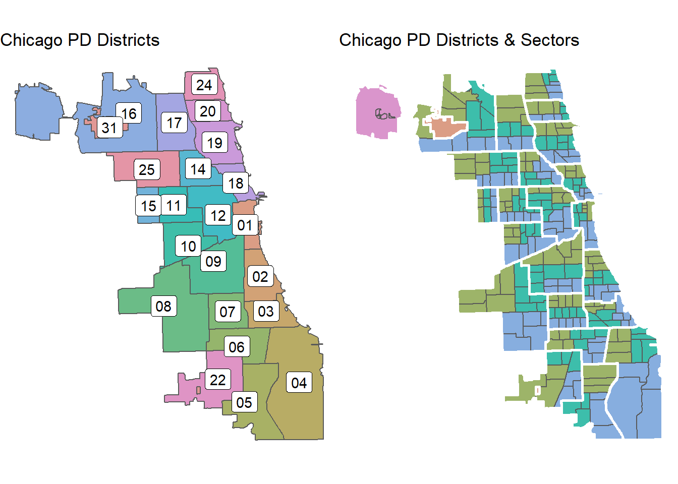
If you want to plot all the beats in Chicago and color in the individual districts (similar to the image above), you can copy-and-paste the following code:
# Plot beats and color in districts
ggplot() +
  geom_sf(data = chicago_beat, aes(fill = district))
Let’s get down to analysis. As usual, we need to focus our attention on a specific region of the city. Let’s choose a district at random - say district 10. We can create a new shapefile using the following code:
# Select District 10
district_10 <- filter(chicago_beat, district == 10)

# Plot District 10, with individual beats
ggplot() +
  geom_sf(data = district_10, aes(fill = beat))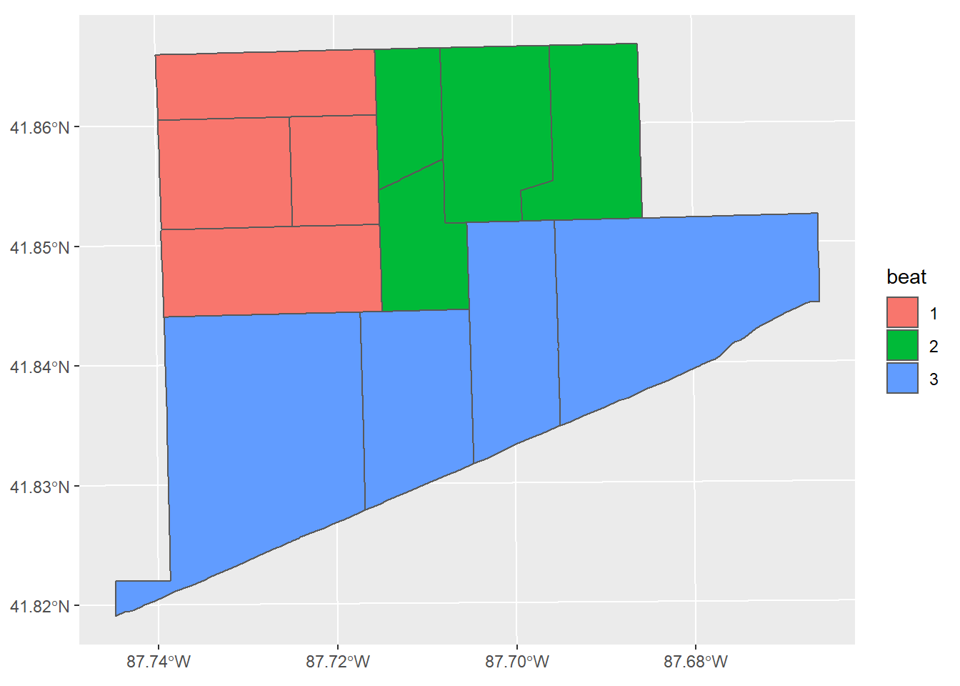
Finally, let’s use a spatial clip to get only the crimes that occurred in district 10 (look back at Lab 8 for a refresher on how the spatial clip works).
# Spatial clip
# Select only crimes within district 10
district_10_crimes <- chicago_crime[district_10,]

# Descriptives of crimes
table(district_10_crimes$crime)
##
## ARSON ASSAULT BATTERY
## 21 1002 2622
## BURGLARY CONCEALED CARRY LICENSE VIOLATION CRIM SEXUAL ASSAULT
## 350 21 39
## CRIMINAL DAMAGE CRIMINAL SEXUAL ASSAULT CRIMINAL TRESPASS
## 1226 28 221
## DECEPTIVE PRACTICE GAMBLING HOMICIDE
## 468 28 34
## INTERFERENCE WITH PUBLIC OFFICER INTIMIDATION KIDNAPPING
## 77 7 8
## LIQUOR LAW VIOLATION MOTOR VEHICLE THEFT NARCOTICS
## 23 468 1886
## OBSCENITY OFFENSE INVOLVING CHILDREN PROSTITUTION
## 1 140 7
## PUBLIC PEACE VIOLATION ROBBERY SEX OFFENSE
## 170 434 71
## STALKING THEFT WEAPONS VIOLATION
## 10 1760 490This gives us two shapefiles now:
- district_10 = boundaries of district 10, with 3 beats
- district_10_crimes = the 12,341 crimes that occurred within district 10
From here on out we are going to focus only on these two shapefiles.
11.2 Selecting Person and Property Crimes
Let’s subset our data a bit further here and separate person and property-related crimes.
For our person-related crimes we’re going to focus on the broad categories of robbery, assault, and homicide.
As we saw above, there are a large number of crimes, but we only want three of them: ROBBERY, ASSAULT,
and HOMICIDE. How do we do this using the filter function? Easy!
We will use the code: crime %in% c("ROBBERY","ASSAULT","HOMICIDE") to filter out ONLY these three crimes.
What this code is telling the computer is essentially:
Look at the variable ‘crime’ and give me ONLY the crimes matching the ones in this list.
We can then save this as a new shapefile called district_10_crimes_person.
district_10_crimes_person <-
  filter(district_10_crimes, crime %in% c("ROBBERY","ASSAULT","HOMICIDE"))
Now we’re ready to plot. We’re going to plot the borders of District 10, the location of the crimes, and color them based on their type. We’ll also add a title:
ggplot() +
  geom_sf(data = district_10) +
  geom_sf(data = district_10_crimes_person, aes(color = crime)) +
  labs(title = "Person-Related Crimes, District 10") +
  theme_void()
This is still a lot of crime to look at. Let’s filter down our data to select only a subset of time. If you look at the data there are a number of time variables to examine including:
month= month of incidentday= day of monthwk_day= day of week
Let’s assume we want to look at only crimes in June, that occurred on Friday through Sunday
We can easily do that using another filter function. Here we’re going to select the month of June using
month == 6 Friday through Sunday doing wk_day %in% c('Fri', 'Sat', 'Sun).
district_10_crimes_person <-
  filter(district_10_crimes_person,month == "Jun", wk_day %in% c('Fri', 'Sat', 'Sun'))
Now let’s plot the new result, updating our title as well:
ggplot() +
  geom_sf(data = district_10) +
  geom_sf(data = district_10_crimes_person, aes(color = crime)) +
  labs(title = "Person-Related Crimes, District 10, Friday - Sunday") +
  theme_void()
Using this, we can see that a lot of the crimes are clustered in the northern region of the district. We might look at the characteristics of the incidents and then formulate a tactical response plan to help deal with the clusters of robberies or assaults that are occurring during the night.
11.3 Other Analyses
At this point, it is up to you on other analyses to perform. Here, maybe we want to also add a hot spot map to identify ‘hot’ and ‘cool’ regions of the district, or maybe we want to see if there are any noteworthy clusters. For example:
11.3.1 Hot spot map
# Load kernel_density
load("C:/Users/gioc4/Desktop/kernel_density.Rdata")
# Create kernel density plot
kde_plot <- kernel_density(district_10_crimes_person, district_10, bdw = 500, plot = FALSE)
# Plot our results
ggplot() +
geom_raster(data = kde_plot, aes(x = X, y = Y, fill = density)) +
geom_sf(data = district_10, fill = NA, color = "white") +
scale_fill_viridis_c()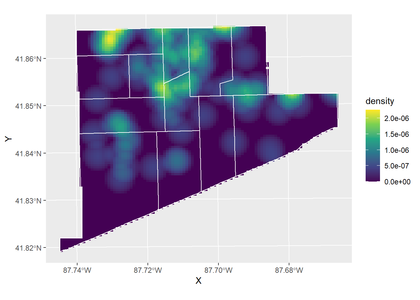
11.3.2 DBscan clusters
# Load cluster_points
load("C:/Users/gioc4/Desktop/cluster_points.Rdata")
# Identify clusters with default values
cluster_points(district_10_crimes_person, district_10)## DBSCAN clustering for 79 objects.
## Parameters: eps = 1000, minPts = 5
## The clustering contains 3 cluster(s) and 57 noise points.
##
## 0 1 2 3
## 57 7 7 8
##
## Available fields: cluster, eps, minPts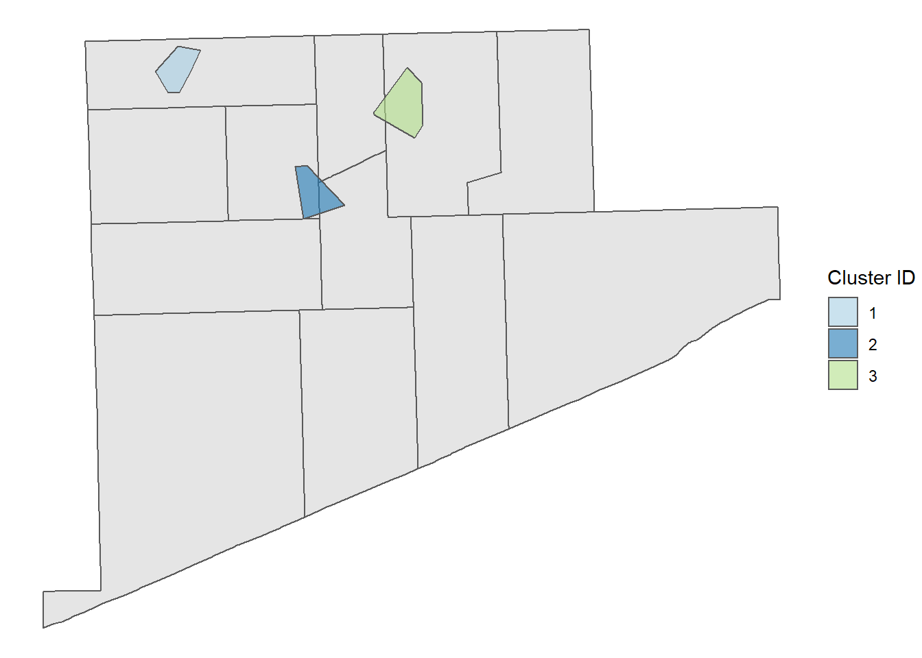
11.4 Lab 9 Assignment
This lab assignment is worth 10 points. Follow the instructions below.
- Using the
chicago_crimedata, filter the data by:- Selecting two or more persons crimes, or property crimes
- Filtering by month, day, or time of day
- Using the
chicago_beatdata, filter the data by:- Selecting one specific district
- Spatially clipping your crime data to that district
- Create the following visualizations:
- A point map showing the locations of your crimes
- A hot spot map showing the location of possible crime hot spots OR
- A graduated color map, coloring locations by police beat OR
- A DBscan cluster map
- Write, in at least one paragraph: Describe any patterns you observe in crimes, based on the crime type you chose, and time(s) you filtered Any tactical-based methods you might apply to prevent further crime problems
In your write up you must include the following: + The two maps created in step 3 + At a minimum one paragraph write-up