Chapter 6 Lab 4 - Working with Variables
Welcome to Lab 4! In this lab we are going to focus on
Topics Covered
- Working with dates
- Plotting spatial data with other variables
- Filtering and subsetting data
- Faceted point maps
6.1 Spatial Data With Variables
Up to now we have relied on shapefiles with no additional data - just the coordinates attached to the shapefile (lat/lon or x/y). However, we often might work with shapefiles that have additional data attached. For instance, if we had a crime incident shapefile, we might also have variables such as:
- The type of building the crime occurred in
- Time of day, or day of week of the crime
- Age or sex of the individuals involved
- The value of any items stolen
In reality, most of the data you work with will have additional data attached to it along with the spatial coordinates. An important part of a crime analyst is to incorporate this data into your analysis. Let’s get started.
To start, let’s open all the libraries we need for this lab: sf, tidyverse
and lubridate. Also, for now on, I will be adding comments to the code. You
should also consider adding comments using the hashtag symbol #. These will
help you understand what you were doing in your code.
Before we start, let’s be sure have lubridate installed.
install.packages("lubridate")Now we can load in all of the tools we will need for this lab.
# Load in libraries
# NOTE: This is a comment!

library(sf)
library(tidyverse)
library(lubridate)
We’ll start by reading in two shapefiles: nyc_shooting.shp and nyc_city.shp. These come from the webpage. Let’s use the function st_read() to read in the shapefile, then save it as a variable so we can work
on it in R. For this example we are going to call our two shapefiles
“shooting” and “city” for simpliciy
# Load in the shapefiles
shooting <- st_read("C:/Users/gioc4/Desktop/nyc_shooting.shp")
city <- st_read("C:/Users/gioc4/Desktop/nyc_city.shp")
The first shapefile shooting has data on every victim of fatal and non-fatal shootings in New York City for the year 2017. The second shapefile city has information about the boundaries and names of each of the 5 boroughs in New York City.
6.1.1 Using glimpse to examine a dataframe
Before we do anything else, we should first look at our data to understand what we’re working with. Let’s try using a new function called glimpse() to look at the variables in the data. Here we see that we have 969 observations
(that is, individual shootings represented as points) and 8 variables.
glimpse(shooting)## Rows: 969
## Columns: 8
## $ id_key <int> 173129246, 173120488, 173120488, 173105454, 173084537, 173084538, 173070862, 173070861, 173035796, 173035796~
## $ date <date> 2017-12-31, 2017-12-31, 2017-12-31, 2017-12-29, 2017-12-29, 2017-12-29, 2017-12-29, 2017-12-28, 2017-12-28,~
## $ year <dbl> 2017, 2017, 2017, 2017, 2017, 2017, 2017, 2017, 2017, 2017, 2017, 2017, 2017, 2017, 2017, 2017, 2017, 2017, ~
## $ boro <chr> "BROOKLYN", "BROOKLYN", "BROOKLYN", "BRONX", "MANHATTAN", "BROOKLYN", "BRONX", "MANHATTAN", "BRONX", "BRONX"~
## $ vic_race <chr> "BLACK", "BLACK", "BLACK", "BLACK", "BLACK", "WHITE HISPANIC", "BLACK", "ASIAN / PACIFIC ISLANDER", "BLACK",~
## $ vic_sex <chr> "M", "M", "M", "M", "M", "M", "M", "M", "M", "M", "M", "M", "M", "M", "M", "M", "F", "M", "M", "M", "M", "M"~
## $ vic_age <chr> "18-24", "18-24", "25-44", "25-44", "18-24", "18-24", "<18", "25-44", "<18", "<18", "<18", "18-24", "18-24",~
## $ geometry <POINT [m]> POINT (1833140 561221.1), POINT (1830159 574401.4), POINT (1830159 574401.4), POINT (1833079 585311.2)~Among the variables we have a unique identifier id_key, a date and year variable. A variable boro which reports which borough the shooting occurred
in, and information on the victim’s race, sex, and age (vic_race, vic_sex, vic_age). Finally, the geometry variable contains information about the
exact longitude and latitude of the data.
glimpse(city)## Rows: 5
## Columns: 5
## $ boro_code <dbl> 1, 2, 5, 3, 4
## $ boro_name <chr> "MANHATTAN", "BRONX", "STATEN ISLAND", "BROOKLYN", "QUEENS"
## $ shape_area <dbl> 636600558, 1186612483, 1623920682, 1937566944, 3044771591
## $ shape_leng <dbl> 361649.9, 462958.3, 330432.9, 739945.4, 895229.0
## $ geometry <MULTIPOLYGON [m]> MULTIPOLYGON (((1826629 569..., MULTIPOLYGON (((1833064 583..., MULTIPOLYGON (((1826427 555..., MULTIPOLYG~The city shapefile has 5 variables, but most of them aren’t of much help to us.
We do have an identifier called boro_name which will come in handy later.
6.1.2 Using summary to examine variables
Because we’re working with variables now, we will want to know some information about them. One function we can use is called summary(). This function gives
you a breakdown of the variables inside a data frame. For instance, we can look
at a number of things inside the shooting data frame.
summary(shooting)## id_key date year boro vic_race vic_sex
## Min. :159826972 Min. :2017-01-01 Min. :2017 Length:969 Length:969 Length:969
## 1st Qu.:164301441 1st Qu.:2017-04-28 1st Qu.:2017 Class :character Class :character Class :character
## Median :166886662 Median :2017-07-07 Median :2017 Mode :character Mode :character Mode :character
## Mean :166899952 Mean :2017-07-09 Mean :2017
## 3rd Qu.:169761148 3rd Qu.:2017-09-25 3rd Qu.:2017
## Max. :173129246 Max. :2017-12-31 Max. :2017
## vic_age geometry
## Length:969 POINT :969
## Class :character epsg:NA : 0
## Mode :character +proj=aea ...: 0
##
##
## Here we see information about the attributes of some variables including the
boro variable. We can see that, for instance, 305 shootings occurred in the
Bronx, while 357 shootings occurred in Brooklyn. We can also see some victim characteristics. The variable vic_sex shows that 885 victims were male,
while 84 were female. Knowing these variables will come in handy later
because we will need them to use for filtering.
6.2 Plotting Shapefiles with ggplot
Now that we have our data examined, let’s start by using ggplot to look
at the distribution of shootings across the five boroughs of New York City.
# Plot out shootings in NYC
ggplot() +
  geom_sf(data = city) +
  geom_sf(data = shooting)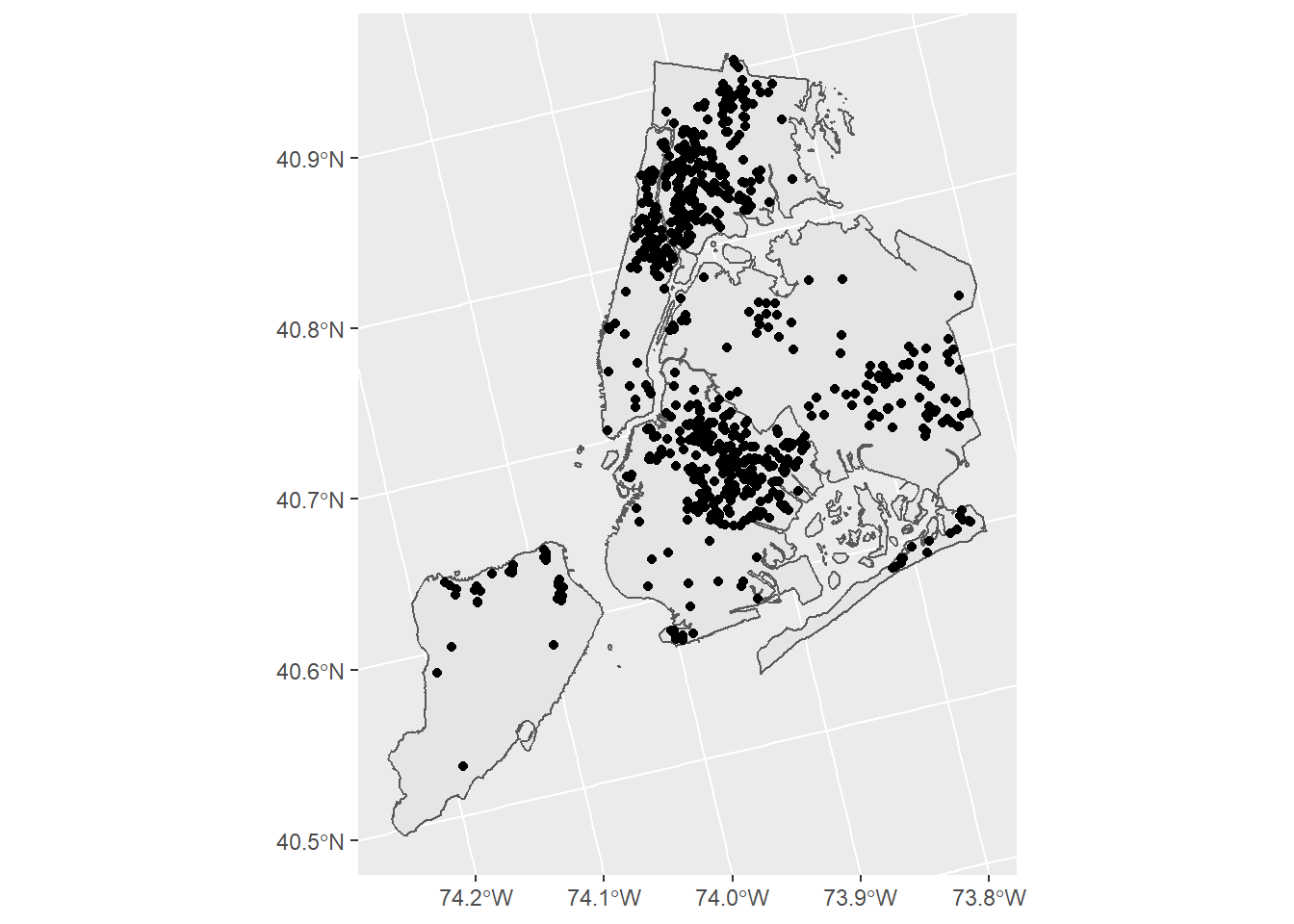
The map above is a little messy, so we can try and clean it up. As always,
we will probably want to change the shape and color of our points and polygons.
This will help us visualize the points better. Remember, you can type in
colors()in the console to get a list of many different named colors
available in R.
ggplot() +
  geom_sf(data = city, fill = "wheat", color = "white") +
  geom_sf(data = shooting, shape = 3, color = "darkseagreen")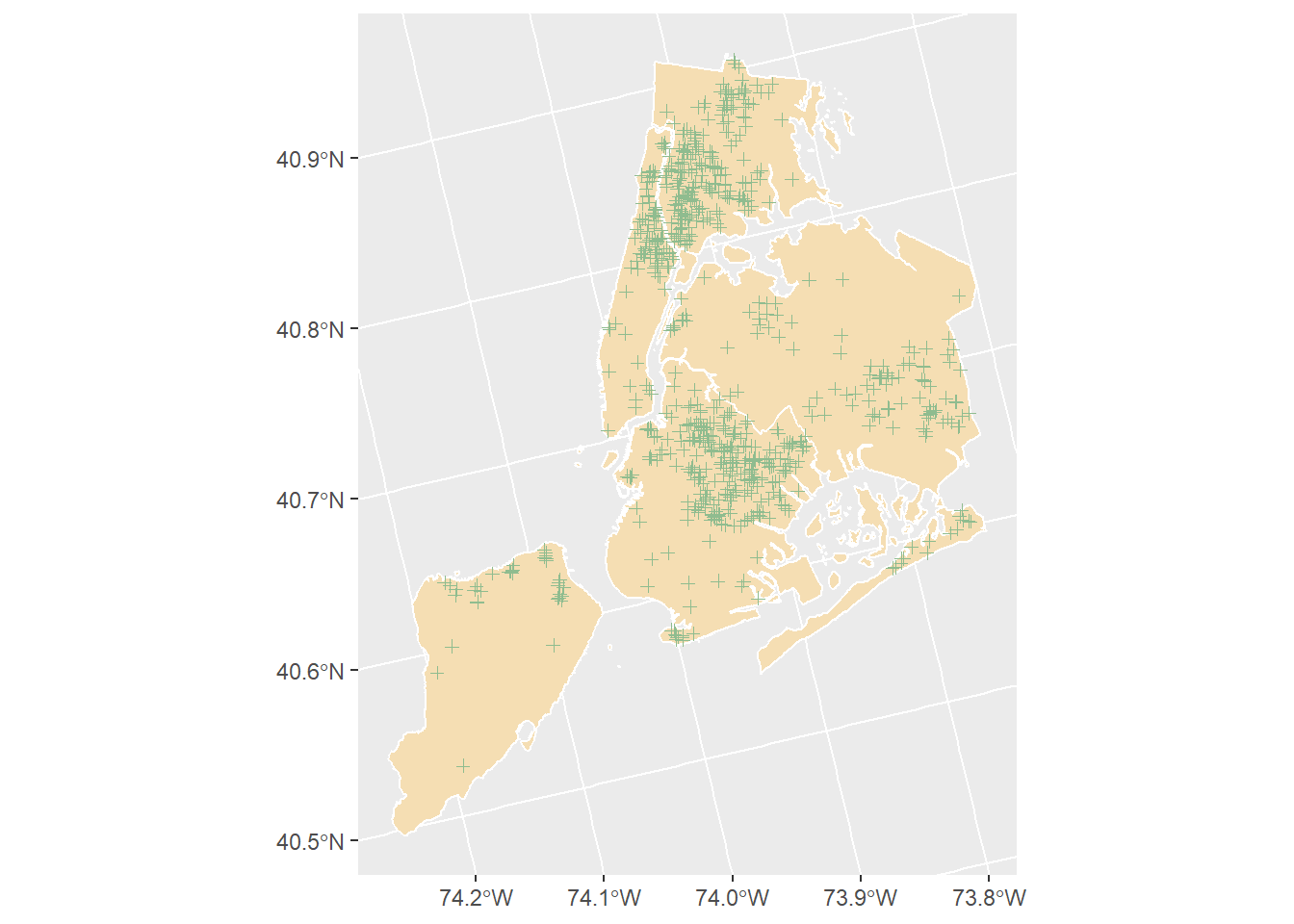
6.3 Filtering and Subsetting Variables
In the above examples we obviously have a lot more data than is useful. Maybe we want to try and perform an analysis on a smaller subset of the data? For instance, imagine the chief of police asked you to:
- Plot only shootings that occurred in Brooklyn
- Create a point map of all shootings in March
To do this, we need to create smaller subsets of data to plot. For this, we are going to use the function filter. The function filter lets us remove or
retain observations based on their values on one or more variables.
For instance, let’s say we want only shootings that occurred in Brooklyn. First,
let’s use the command unique to look at the unique attributes in the variable boro.
# Find all the unique values of 'boro'
unique(shooting$boro)
## [1] "BROOKLYN" "BRONX" "MANHATTAN" "STATEN ISLAND" "QUEENS"So, we see the variable boro is the name of the borough in which the shooting
occurred. The attributes for this variable are all capitalized as well (keep
this in mind!). The filter function allows us to select only the rows in the
data that meet one or more requirements. Look at this image below:
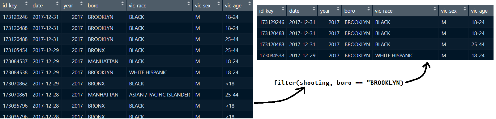
Figure 6.1: Applying the filter function
You can see that the filter function has left us with only those shootings
where boro == BROOKLYN. The double equals sign == just tells R that we want
to test if something is equal to a value.
Now, to do this for our analysis, all we have to do is save the output of this function into R. Let’s try it out and then we’ll look at what happened.
# Filter only shootings in Brooklyn
shooting_brooklyn <- filter(shooting, boro == "BROOKLYN")
Let’s break down what’s happening here:
- Create a new variable named
shooting_brooklyn - Use the
filter()function on the shapefile,shooting - Specify that we only want shootings that occurred in Brooklyn
Importantly here, the == sign means that we want only the values that are
equal to BROOKLYN. Let’s try plotting the results of this
# Plot just the shootings in Brooklyn
ggplot() +
  geom_sf(data = city, fill = "wheat", color = "white") +
  geom_sf(data = shooting_brooklyn, shape = 3, color = "darkseagreen")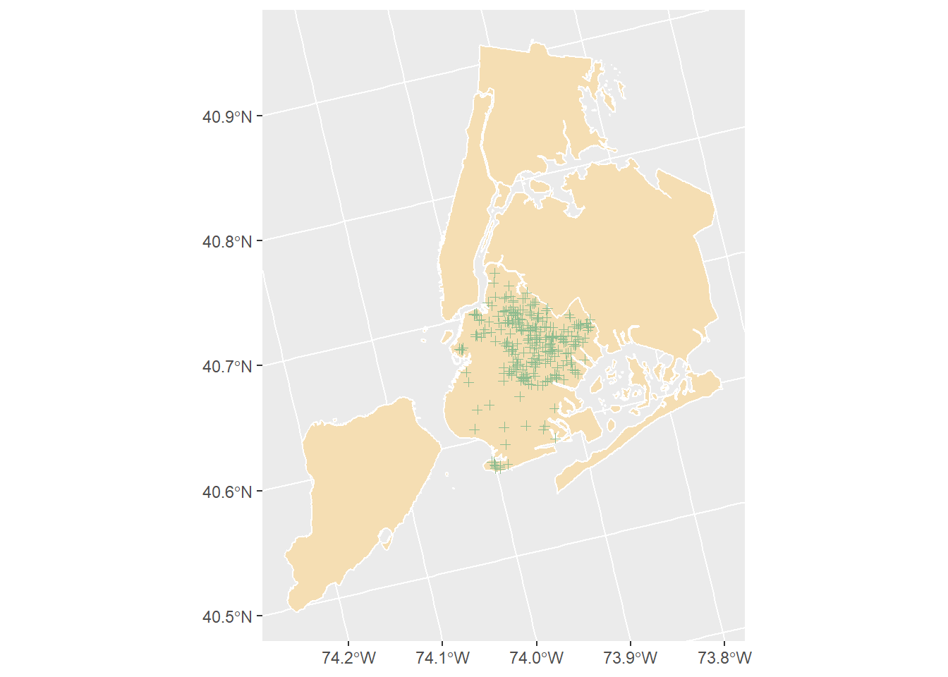
Now we have just the shootings that occurred in Brooklyn. But our map still has
all the other boroughs in it! How can we get rid of them? With filter of
course! Let’s filter the other shapefile city and get just Brooklyn.
For this, we’ll call the new shapefile, brooklyn. Also, note that in the
city shapefile, the variable that stores the name is called boro_name and
not boro. You can check this manually by doing glimpse(city) first.
# Get only the polygon for Brooklyn
brooklyn <- filter(city, boro_name == "BROOKLYN")
And now we can plot it again, replacing the file city with brooklyn
# Plot just the shootings in Brooklyn
ggplot() +
  geom_sf(data = brooklyn, fill = "wheat", color = "white") +
  geom_sf(data = shooting_brooklyn, shape = 3, color = "darkseagreen")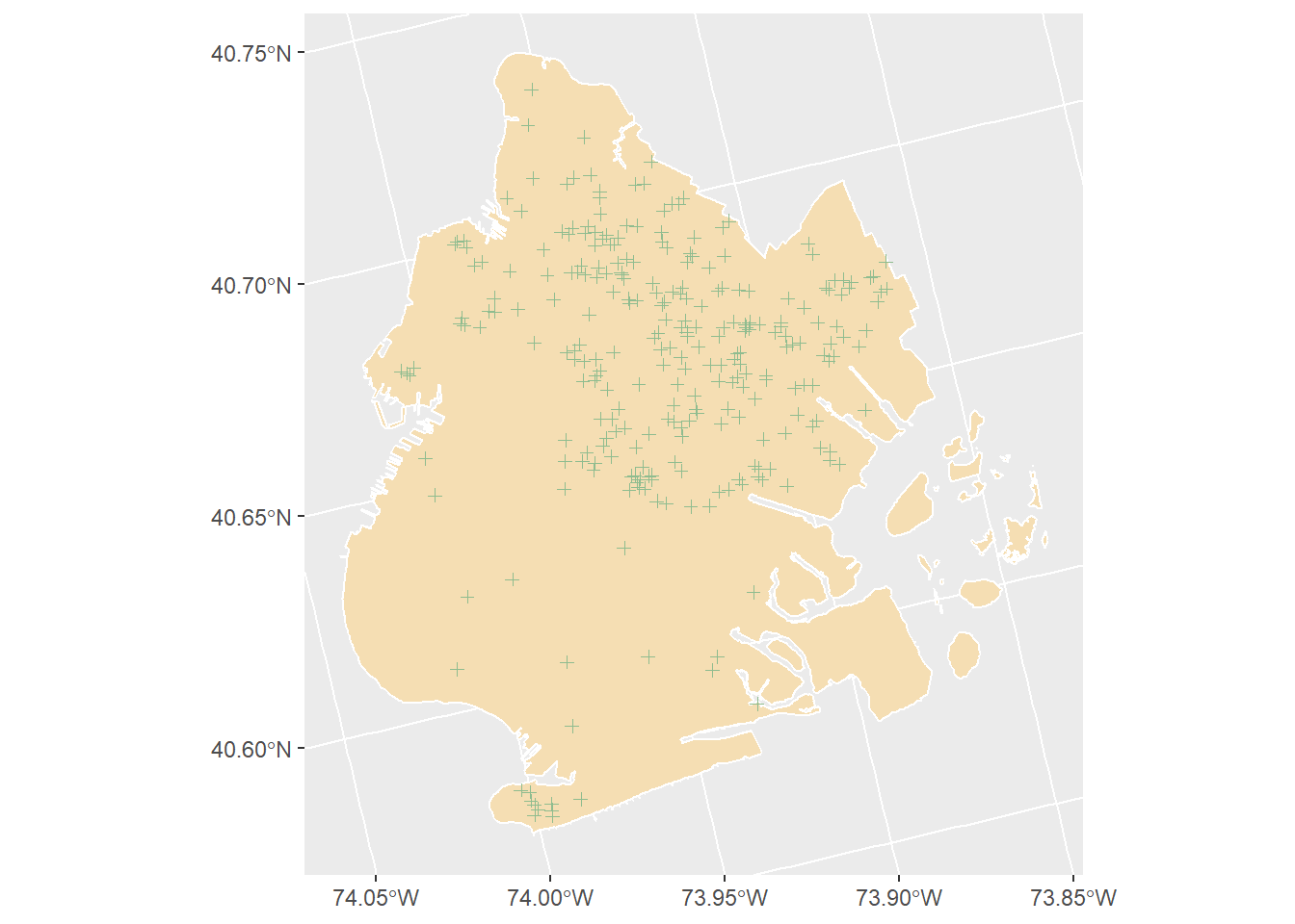
Now, what if we want to filter all shootings in Brooklyn and only shootings
that occurred in the month of March? To do this, we can just add another
argument to the filter() function we used above. The variable we want to
filter by is called date, which reflects the date that the shooting
occurred on. However, working with dates requires a bit of special work. Let’s
discuss.
6.4 Working with dates
One of the types of data we will be working with is a date variable.
Dates in R are always represented as yyyy-mm-dd. To help working with date variables we are going to utilize a specific package called lubridate. The lubridate package is simply a set of tools
that make working with date variables easier.
head(shooting$date)## [1] "2017-12-31" "2017-12-31" "2017-12-31" "2017-12-29" "2017-12-29" "2017-12-29"This shows that the date variable is just a collection of dates in year-month-date format. What do we want to do if we just want the month that the incident occurred in. We can use the function month() that is part of the lubridate package!
head( month(shooting$date) )## [1] 12 12 12 12 12 12So if we do month(shooting$date) we will get the number (1 - 12) that the month occurred in. Let’s use the filter function to filter both the date and the
borough (which we did above).
# Filter only the shootings in March
# AND only in Brooklyn
shooting_march_brooklyn <- filter(shooting, month(date) == 3,
                                  boro == "BROOKLYN")
And if we plot the result of this we get:
# Plot just the shootings in Brooklyn
ggplot() +
  geom_sf(data = brooklyn, fill = "wheat", color = "white") +
  geom_sf(data = shooting_march_brooklyn, shape = 3, color = "darkseagreen")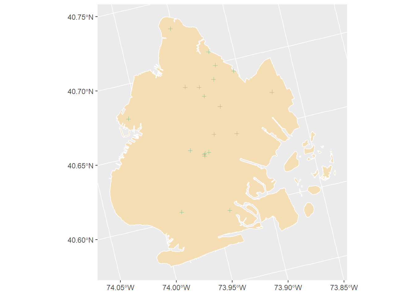
Finally, let’s clean up our plot. I want to remove the grey background, increase the size of the points, and add a descriptive title.
# Plot just the shootings in Brooklyn
ggplot() +
  geom_sf(data = brooklyn, fill = "wheat", color = "white") +
  geom_sf(data = shooting_march_brooklyn, shape = 3, size = 2, color = "darkseagreen") +
  labs(title = "Shootings in Brooklyn, March 2017") +
  theme_void()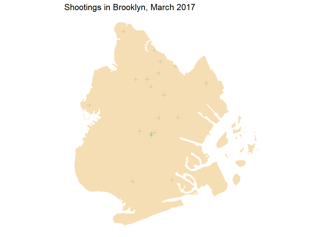
6.5 Lab 4 Assignment
This lab assignment is worth 10 points. Follow the instructions below.
On your own, load the two shapefiles nyc_shooting.shp and nyc_city.shp
- Create a new dataframe using the shapefile
shootingsby usingfilter()on one of the following variables:- vic_race
- vic_sex
- vic_age
- In the shapefile
shootings, also usefilter()to select one of the following boroughs:- “BRONX”
- “BROOKLYN”
- “MANHATTAN”
- “QUEENS”
- “STATEN ISLAND”
- In the
cityshapefile usefilter()to select one of the following boroughs (note, this should be the same that you chose above):- “BRONX”
- “BROOKLYN”
- “MANHATTAN”
- “QUEENS”
- “STATEN ISLAND”
- Generate a new point map using your filtered
shootingandcitydata frames. Be sure to include the following:- Selected points
- Selected borough
- New colors, shapes, and sizes for points
- New colors for borough
- For question 4 include a 1-paragraph write-up. Write:
- The variable you filtered and the borough you chose
- Note the general location and distribution of crimes
- Speculate on any patterns you observe, and possible ways to investigate further