Chapter 5 Lab 3 - What is a hot spot?
Welcome to Lab 3! In this lab we are going to focus on
Topics Covered
- Plotting a point map
- Loading in the
kernel_densityfunction - Creating a hot spot map
- Experimenting with different bandwidths
5.1 Loading your data
To begin, we’re first going to load three different sets of data into R. These are all spatial datasets, so we will
need to use the function st_read. Before we do anything else, we should load our libraries into R. We will need the
tidyverse package to do some of the plotting, and the sf package to handle our spatial data.
library(tidyverse)
library(sf)
Now that we have our libraries loaded in, we can start. Let’s start by loading our two datasets in: the New Haven data and the burglary data.
new_haven <- st_read("C:/Users/gioc4/Desktop/nh_blocks.shp")
burglary <- st_read("C:/Users/gioc4/Desktop/nh_burglary.shp")
Now that we’ve loaded them in, we should start by creating a small point map to evaluate the distribution of burglaries
across New Haven. Remember from the previous lab, we will do this using ggplot and the function geom_sf.
5.2 Evaluating a point map
Here’s a basic point map, with the fill and colors changed (remember, try typing in colors() in the console to get)
ggplot() +
  geom_sf(data = new_haven, fill = "powderblue") +
  geom_sf(data = burglary, color = "violetred2")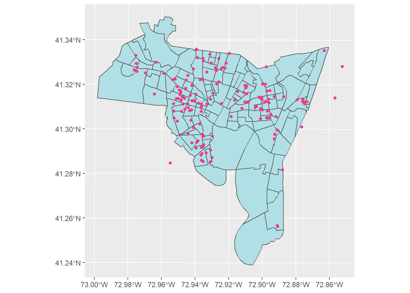
5.3 Kernel density mapping
What is kernel density mapping? In effect, it is a method to calculate the relative density of points in a region. It has many applications, but in criminology we are primarily interested in identifying crime ‘hot-spots.’ We can conceptualize these as being regions with a high density of crimes relative to other places in a city. The ‘kernel’ in kernel density mapping is a small window that we pass over each of the points. For each point we calculate a density value in that point’s neighborhood. We repeat this process for each point to give us a map of densities (see below).
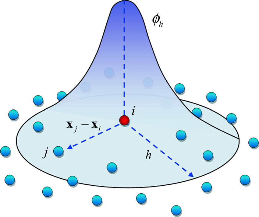
Figure 5.1: Passing a kernel over a group of points
How can we calculate this in R? Well, there are a number of options but luckily for us there is a bit of code (written
by yours truly). Let’s talk about a tool we can use called the kernel_density function.
5.3.1 The kernel_density function
You might have noticed a file named kernel_density.Rdata. This is a code fragment that you can load into R and then
use to run. In this case, the code will handle a lot of the work needed to make a kernel density map. When you see a
file with .Rdata attached to it, you can use the load function to load it into R. Let’s try loading this function now.
load("C:/Users/gioc4/Desktop/kernel_density.Rdata")Now that you’ve loaded this into R, you can use the kernel density function to perform some actions for you. In short, this function will allow you to take a set of points and polygons and calculate a hot spot map. All you have to do is fill in some information. Let’s go over the options:
- The function
kernel_densitytakes the following arguments:- point_data = The point data (usually crimes) that you want to use
- polygon_data = The boundaries of the location you are studying
- bdw = The bandwidth (in feet) that you will use as your search radius
- npixel = The size of the pixels in your hot spot map. Larger n = smaller pixels
- plot =
TRUEorFALSEif you want a quick plot (TRUEby default) - area =
TRUEorFALSEif you want the size of each pixel (in feet) returned (FALSEby default)
However, all we need to do at a minimum is specify what our point data is, and what our polygon data is. Here, our point
data is the location of burglaries (burglary) and our polygon data is the boundaries of New Haven (new_haven). We
are also going to save this as object so we can use it later. Let’s call it kde_burglary, because it is our kernel
density estimate (KDE) for burglaries.
kde_burglary <-
  kernel_density(point_data = burglary, polygon_data = new_haven)
## [1] "Calculating bandwith..."
## [1] "Bandwidth: 1870.3"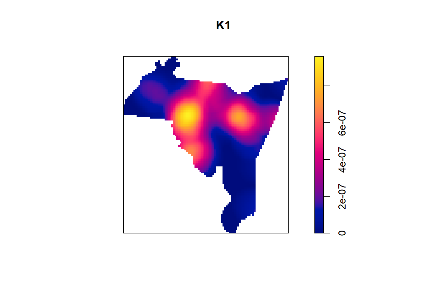
And there we go! By default kernel_density will automatically estimate a bandwidth for you (remember, the
bandwidthcontrols how large the kernel is). In addition, it will provide you with a small picture of the plot.
However, we willlikely want to make a prettier image, so we will just use this for diagnostic purposes.
Before we go any farther, let’s discuss how to choose a bandwidth.
5.3.2 Choosing a bandwidth
In general, the larger the bandwidth, the smoother the image will be. The smaller the bandwidth, the tighter it will
be around individual points. We want to try and find a value that balances smoothness while not over-smoothing. Let’s
look at two different bandwidth sizes and compare. One I will set to 1000 feet and the other I will set to 5000 feet).
In addition, I will save them as two separate objects, so we can compare later. One will be named kde_burglary1000 and
the other will be named kde_burglary5000.
Here is the 1000 foot bandwidth:
kde_burglary1000 <-
  kernel_density(point_data = burglary, polygon_data = new_haven, bdw = 1000)
…and the 5000 foot bandwidth:
kde_burglary5000 <-
  kernel_density(point_data = burglary, polygon_data = new_haven, bdw = 5000)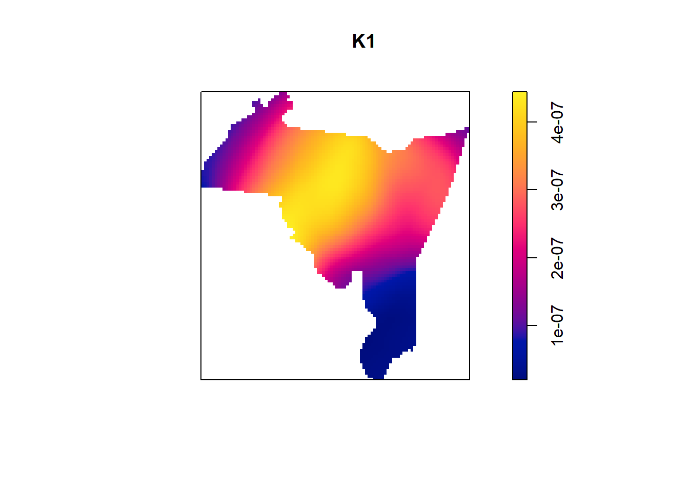
Here we can see the difference that bandwidth size makes. A small bandwidth (1000 feet) seems to generate some easily identifiable hot spots, while not over-smoothing the map. 5000 feet is likely too large, as the map is completely smoothed over. It will be up to you, as the analyst, to determine a bandwidth that helps identify patterns of hotspots. You should try several and choose the one that best highlights the patterns.
5.4 Plotting your map in ggplot
While the diagnostic plots above are helpful, we do want to professionalize our plots. Let’s take the data from one of
our kernel density estimations and use ggplot to make a pretty plot for us. Here, we can just add the data to a
geom in ggplot. However, instead of an sf value (which is vector data) we have a raster file! So instead we will use
a geom_raster and provide the x and y coordinates for our plot. Additionally, we’ll add in the fill of the raster
based on the density estimated in the kernel density program. Let’s see what that looks like in R code:
ggplot() +
  geom_sf(data = new_haven, fill = NA) +
  geom_raster(data = kde_burglary1000, aes(x = X, y = Y, fill = density))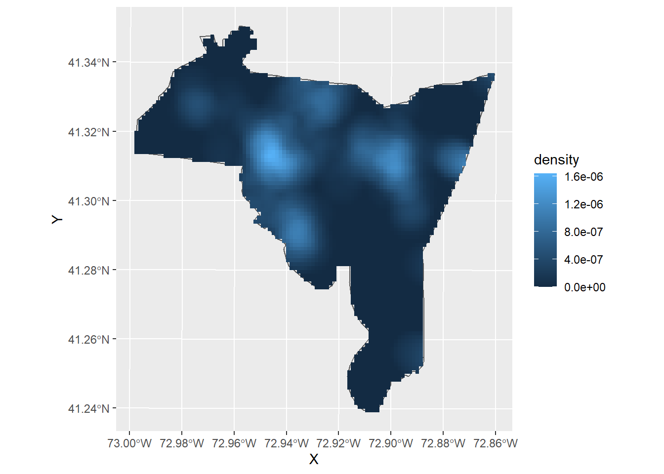
Lets change the color scheme. We can utilize the built-in viridis color scheme to help better highlight the patterns. All you have to do is add the code scale_fill_viridis_c()
at the end of your ggplot to change the fill color to the viridis scale.
ggplot() +
  geom_sf(data = new_haven, fill = NA) +
  geom_raster(data = kde_burglary1000, aes(x = X, y = Y, fill = density)) +
  scale_fill_viridis_c()
A properly-formatted, finished map might look something like this. Here, we’ve added a title and removed the grey
background using the command + theme_void()
ggplot() +
  geom_sf(data = new_haven, fill = NA) +
  geom_raster(data = kde_burglary1000, aes(x = X, y = Y, fill = density)) +
  labs(title = "Burglary Hot Spots in New Haven") +
  scale_fill_viridis_c() +
  theme_void()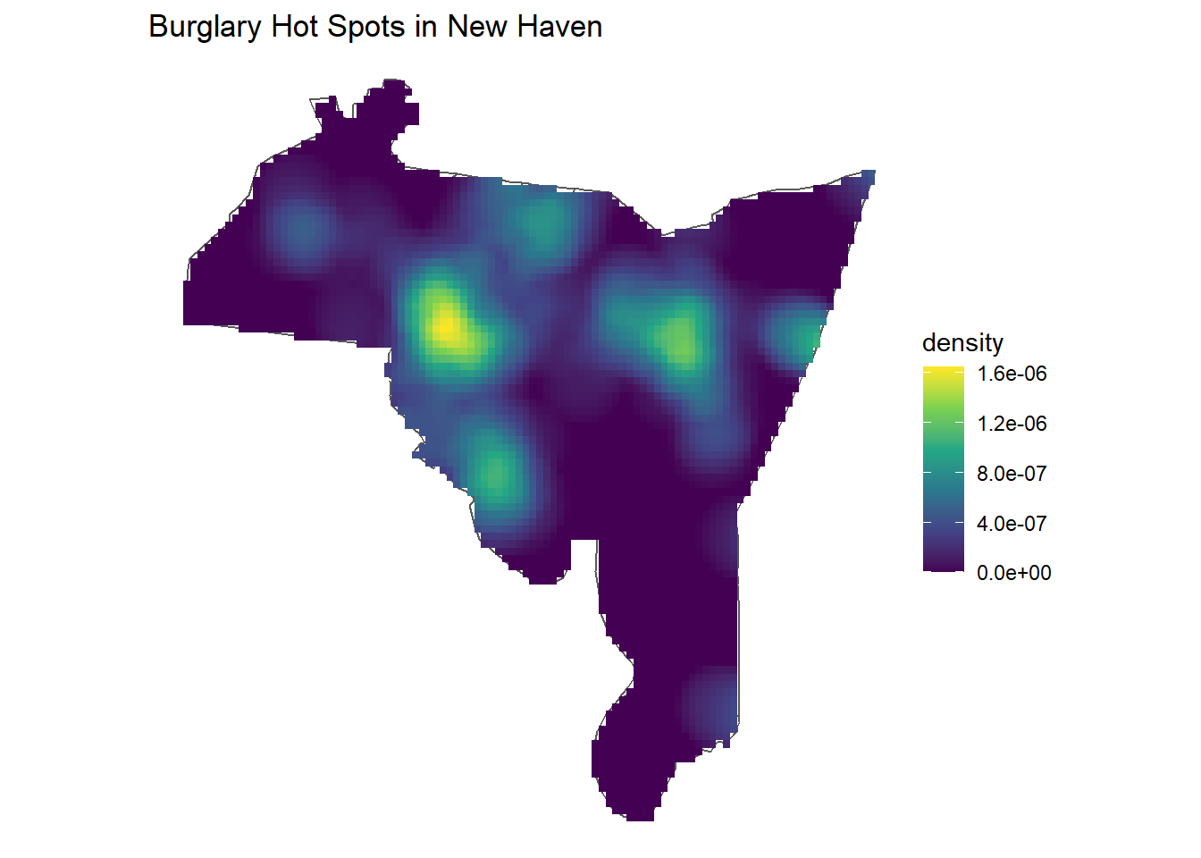
5.5 Lab 3 Assignment
This lab assignment is worth 10 points. Follow the instructions below.
- Use the function
st_readto load the shapefilesnh_blocksandnh_burglaryinto R- Create a simple point map, using custom colors, shapes, and sizes
- Load the
kernel_densityfunction into R usingload- Create a hot spot map using a custom bandwidth size
- Plot your hotspot map using the
ggplotfunction
- In at least one paragraph, describe the distribution of burglary incidents in New Haven. Discuss the size of the bandwidth you chose for your hot spot map. Discuss why you chose that specific size, and how it compares to other bandwidth sizes you might have chosen