Chapter 3 Lab 1 - Getting Started with R
Welcome to Lab 1! In this lab, we will be focusing on a few, very basic issues. Below, you will see a list of the major topics that will be covered. Every lab will have a list of the major skills you will be learning.
Topics Covered
- Introduction to RStudio
- Installing packages
- Loading data into
R - Working with variables
- Plotting spatial data
3.1 Introduction to RStudio
After installing both the R programming language AND Rstudio (hint, if you haven’t done this already please go here and here first).
You should open Rstudio by double clicking on the Rstudio icon. You should be greeted with something that looks like
this:
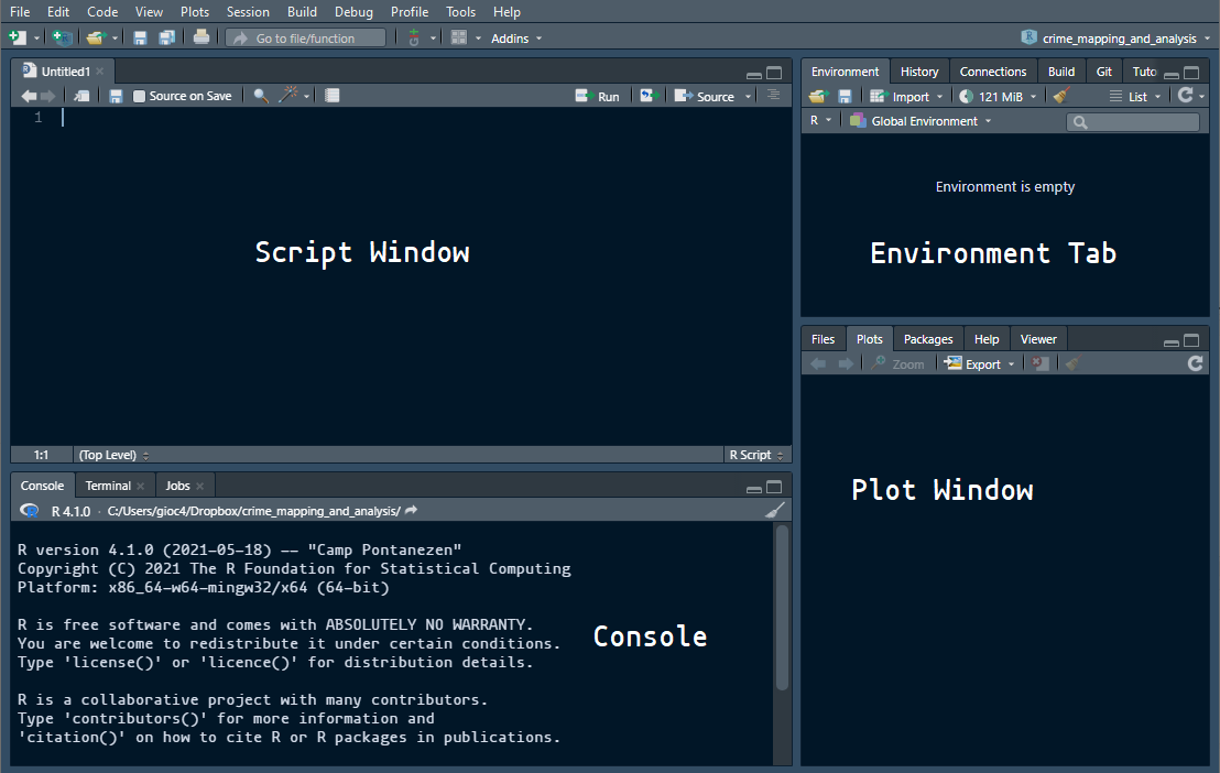
Figure 3.1: The RStudio Interface
The first thing you will want to do is to create a new script. A script is just a list of instructions you will be giving to the computer - like a text document. To start, go to the file window and select ‘New File > R Script.’ A new window should pop up in the top left corner. You will be doing all your work here, in the script window.
You can write and run commands in the editor. Let’s start with some basic math. Trying typing in the following:
2 + 2After typing it in, hit either ctrl+enter (on PC) or command+return (on Mac) to run the code. You should see the results below in the console window.
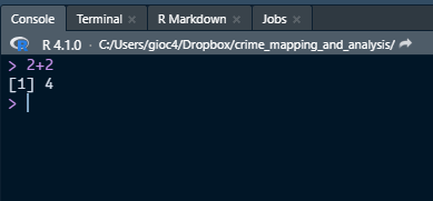
Figure 3.2: Console output
The console window will print out the results of your code. As you will see a little later, we can use the console window to view the results of our commands, as well as any errors or other messages given to us by R.
3.2 Installing packages
The first thing we need to do is to install some packages. In R, a package is a collection of tools that we can use to analyze data. Some of these tools will help us examine spatial crime data, others will help us process data. In R it is quite easy to install these packages and we only need to do it once. There are a few packages we will need to install first. The most important ones are as follows:
tidyverse: A collection of tools making working with data easiersf: A package used to read and process spatial dataspatstat: A spatial statistics packagemaptools: Miscellaneous tools for editing spatial dataraster: A package for plotting ‘raster’ based data
Let’s start by installing the first one, tidyverse. This is very popular package in R and is primarily used to
handle all kinds of data (see here for more information). To install a package, all we
need to do is specify some code. The command in R is install.packages. All we have to do is provide the name of the
package we want to install. Let’s try it.
install.packages("tidyverse")This will likely run for a bit on your computer, then finally stop. After it’s finished, you’re done! You will be
able use all the tidyverse tools in R whenever you want. We will actually use some of these below in a minute. Now,
you should finish installing the rest of the packages. Copy and paste the following code and run it in your script
window. This may take a while (depending on your computer) but you only need to install these one time.
install.packages("sf")
install.packages("spatstat")
install.packages("maptools")
install.packages("raster")
After installing these packages, we just need to load them into R. To do that, we use the function library to load
our tools. Unlike install.packages we need to use library every single time we close and open R. Right now, we
will need the tools from the tidyverse package - so let’s load it in:
library(tidyverse)Now we’re ready to try loading some of our data into R!
3.3 Loading data into R
Loading data into R might seem daunting, but it is actually quite easy once you figure out how it works. All you have to do is specify two things!
- The name of the file you want to load into R.
- The address of the file on your computer.
On a computer, each file has an address. This is just the location where the file is located. To load a file into R you need to provide the computer the address and name of the file. Below, I have the first file shown on my computer, a .csv file named ‘usa_arrests.’ As an aside, a .csv file (also known as a comma-separated values file) is just a way computers commonly store tabular data.
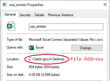
Figure 3.3: File Address of a .csv File
On my computer, my username is ‘gioc4’ and the file is located on my Desktop. The full address of the file is “C:/Users/gioc4/Desktop/usa_arrests.csv.” Now, let’s try and load this into R. Before we do that, we need to talk about an important tool: the assignment operator
3.3.1 The assignment operator
In R, we will often be saving the results of our analyses as objects that we can access later. Think of these as individual files that we can work with (like a word document). We create a name for our object, then save some data into it. That’s where the assignment operator comes in.
In R, we save data using the arrow icon: <-. It’s just a greater-than sign < and a minus sign - next to each
other. Whenever we want to save some data as an object, we use the arrow key pointing toward it. For example:
name_of_variable <- some_dataOn the left-hand side is the name of the object or variable. We put the arrow pointing toward it to save our data as that name, then put the actual data on the right-hand side. Now we’re ready to start.
3.3.2 Using read_csv to load a .csv file
Let’s start by loading a .csv file into R. You should have placed the file usa_arrests.csv onto your dekstop
(or somewhere else where you can point the computer to it). Putting together what we discussed above, we are going to
do the following:
- Define a name for our object
- Use the assignment operator to save data into our new object
- Use the R function
read_csvto import the data into R
The R function read_csv will import our data into R for us. All we have to do is provide the address to the file on
our computer. Once you’re done, your code should look something like this (with the user name changed, of course).
arrests <- read_csv("C:/Users/gioc4/Desktop/usa_arrests.csv")Breaking it down, each piece of this code does this:
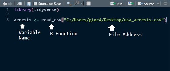
Figure 3.4: Reading a .csv file into R
As you can see, we chose the name arrests for our object name, we used the R function read_csv to load a .csv file,
and then provided (in quotes) the location of the file on our computer.
If you don’t know what your user name is, you can type the following in the console window and hit ‘enter’
getwd()## [1] "C:/Users/gioc4/Dropbox/crime_mapping_and_analysis"The beginning part of this will tell you what your username is. Here you can see my username is ‘gioc4.’
If everything went correctly, you should see the following in the top-right corner of your RStudio window in the environment tab. That’s our data!
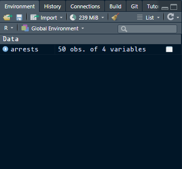
Figure 3.5: Data in the environment tab
3.4 Working with variables
Now that we’ve successfully loaded our data into R, we can start using some data analysis functions to look at it. We have access to a lot of tools to analyze our data. Let’s look at a few.
3.4.1 head and glimpse
First, we can examine the variables in our dataset in order to get an idea of what we’re working with. Two functions,
head and glimpse can help us with that. Let’s first try using the head function on our dataset.
head(arrests)## # A tibble: 6 x 4
## Murder Assault UrbanPop Rape
## <dbl> <dbl> <dbl> <dbl>
## 1 13.2 236 58 21.2
## 2 10 263 48 44.5
## 3 8.1 294 80 31
## 4 8.8 190 50 19.5
## 5 9 276 91 40.6
## 6 7.9 204 78 38.7Here, head gives us the top 6 rows in our dataset, along with the names of the variables. The function glimpse
will work in a similar way, but slightly more consice way.
glimpse(arrests)## Rows: 50
## Columns: 4
## $ Murder <dbl> 13.2, 10.0, 8.1, 8.8, 9.0, 7.9, 3.3, 5.9, 15.4, 17.4, 5.3, 2.6, 10.4, 7.2, 2.2, 6.0, 9.7, 15.4, 2.1, 11.3, 4~
## $ Assault <dbl> 236, 263, 294, 190, 276, 204, 110, 238, 335, 211, 46, 120, 249, 113, 56, 115, 109, 249, 83, 300, 149, 255, 7~
## $ UrbanPop <dbl> 58, 48, 80, 50, 91, 78, 77, 72, 80, 60, 83, 54, 83, 65, 57, 66, 52, 66, 51, 67, 85, 74, 66, 44, 70, 53, 62, ~
## $ Rape <dbl> 21.2, 44.5, 31.0, 19.5, 40.6, 38.7, 11.1, 15.8, 31.9, 25.8, 20.2, 14.2, 24.0, 21.0, 11.3, 18.0, 16.3, 22.2, ~3.4.2 summary
We can also easily get the summary statistics for one, or all of our variables using the summary function.
If we want to examine a single variable inside of our dataset, we need to use the dollar sign $ to access it.
So if I want to get summary statistics on the variable Murder I should do:
summary(arrests$Murder)## Min. 1st Qu. Median Mean 3rd Qu. Max.
## 0.800 4.075 7.250 7.788 11.250 17.400This will give us the minimum, maximum, median, mean, and 1st and 3rd quartiles of the data. Here we see the average murder rate in this dataset is 7.78 per 100,000.
We can also get summary statistics on all the variables at the same time, by just putting in the name of the data object.
summary(arrests)## Murder Assault UrbanPop Rape
## Min. : 0.800 Min. : 45.0 Min. :32.00 Min. : 7.30
## 1st Qu.: 4.075 1st Qu.:109.0 1st Qu.:54.50 1st Qu.:15.07
## Median : 7.250 Median :159.0 Median :66.00 Median :20.10
## Mean : 7.788 Mean :170.8 Mean :65.54 Mean :21.23
## 3rd Qu.:11.250 3rd Qu.:249.0 3rd Qu.:77.75 3rd Qu.:26.18
## Max. :17.400 Max. :337.0 Max. :91.00 Max. :46.003.5 Loading and plotting spatial data
Now that we’re comfortable loading .csv files, let’s move onto files that have spatial data attached. The most common way we encounter spatial data, is through something called a shapefile. A shapefile is:
“a geospatial vector data format for geographic information system software”
Essentially, it is a collection of files that store information about spatial data. For example - it might be the boundaries of a city, or the location of crimes in a city. As you will see below, shapefiles are a bit special because they are a collection of files. Each file has its own purpose, and together they make up all the data needed to plot an object. Look below:
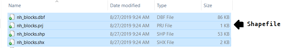
Figure 3.6: Data in the environment tab
In R, we will load shapefiles much the same way we do with a .csv file. However, instead of read_csv we will
use st_read in the sf package. Just like we did above with with read_csv we will do the exact same thing.
We just need to point the computer to the location of the shapefile on our computer. Note: While a shapefile is a
collection of files, we only need to point the computer to the file with the .shp after it.
library(sf)

new_haven <- st_read("C:/Users/gioc4/Desktop/nh_blocks.shp")
Now that its loaded it, we can try plotting it. Try out the code below:
plot(new_haven, max.plot = 1)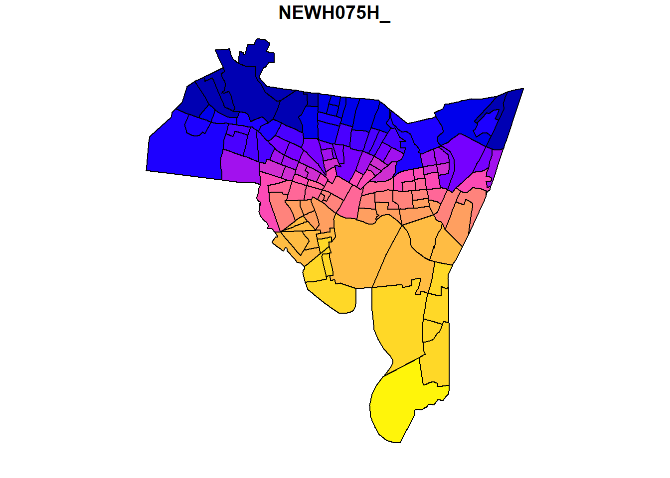
There! Now you’ve succesfully plotted your first shapefile. You can see the colors of the plot correspond to some of
the underlying variables in the shapefile. A shapefile is actually very similar to a normal data file (like a .csv)
except that it has spatial data attached to it. In fact, many of the same functions we used for the .csv file above
will also work here. Let’s see what happens if we use head and glimpse
head(new_haven)## Simple feature collection with 6 features and 28 fields
## Geometry type: POLYGON
## Dimension: XY
## Bounding box: xmin: 534687.6 ymin: 177306.3 xmax: 569625.3 ymax: 188464.6
## Projected CRS: Lambert_Conformal_Conic
## NEWH075H_ NEWH075H_I HSE_UNITS OCCUPIED VACANT P_VACANT P_OWNEROCC P_RENTROCC NEWH075P_ NEWH075P_I POP1990 P_MALES
## 1 2 69 763 725 38 4.980341 0.393185 94.626474 2 380 2396 40.02504
## 2 3 72 510 480 30 5.882353 20.392157 73.725490 3 385 3071 39.07522
## 3 4 64 389 362 27 6.940874 57.840617 35.218509 4 394 996 47.38956
## 4 5 68 429 397 32 7.459207 19.813520 72.727273 5 399 1336 42.66467
## 5 6 67 443 385 58 13.092551 80.361174 6.546275 6 404 915 46.22951
## 6 7 133 588 548 40 6.802721 52.551020 40.646259 7 406 1318 50.91047
## P_FEMALES P_WHITE P_BLACK P_AMERI_ES P_ASIAN_PI P_OTHER P_UNDER5 P_5_13 P_14_17 P_18_24 P_25_34 P_35_44
## 1 59.97496 7.095159 87.020033 0.584307 0.041736 5.258765 12.813022 24.707846 7.888147 12.479132 16.026711 8.555927
## 2 60.92478 87.105177 10.452621 0.195376 0.521003 1.725822 1.921198 2.474764 0.814067 71.149463 7.359166 4.037773
## 3 52.61044 32.931727 66.265060 0.100402 0.200803 0.502008 10.441767 13.554217 5.722892 8.835341 17.670683 17.871486
## 4 57.33533 11.452096 85.553892 0.523952 0.523952 1.946108 10.853293 17.739521 7.709581 12.425150 18.113772 10.853293
## 5 53.77049 73.442623 24.371585 0.327869 1.420765 0.437158 6.229508 8.633880 2.950820 7.103825 17.267760 16.830601
## 6 49.08953 87.784522 7.435508 0.758725 0.834598 3.186646 8.725341 8.194234 3.641882 10.091047 29.286798 12.898331
## P_45_54 P_55_64 P_65_74 P_75_UP geometry
## 1 5.759599 4.924875 4.048414 2.796327 POLYGON ((540989.5 186028.3...
## 2 1.595571 1.758385 3.712146 5.177467 POLYGON ((539949.9 187487.6...
## 3 8.734940 5.923695 7.931727 3.313253 POLYGON ((537497.6 184616.7...
## 4 9.056886 6.287425 4.266467 2.694611 POLYGON ((537497.6 184616.7...
## 5 8.415301 7.431694 14.426230 10.710383 POLYGON ((536589.3 184217.5...
## 6 7.814871 7.814871 6.904401 4.628225 POLYGON ((568032.4 183170.2...glimpse(new_haven)## Rows: 129
## Columns: 29
## $ NEWH075H_ <dbl> 2, 3, 4, 5, 6, 7, 8, 9, 10, 11, 12, 13, 14, 15, 16, 17, 18, 19, 20, 21, 22, 23, 24, 25, 26, 27, 28, 29, 30~
## $ NEWH075H_I <dbl> 69, 72, 64, 68, 67, 133, 73, 134, 84, 80, 79, 136, 77, 97, 94, 102, 78, 66, 83, 62, 121, 135, 65, 126, 81,~
## $ HSE_UNITS <dbl> 763, 510, 389, 429, 443, 588, 410, 615, 316, 365, 276, 393, 355, 595, 518, 277, 232, 264, 502, 772, 467, 2~
## $ OCCUPIED <dbl> 725, 480, 362, 397, 385, 548, 389, 562, 293, 337, 256, 377, 309, 534, 475, 263, 194, 237, 459, 730, 441, 2~
## $ VACANT <dbl> 38, 30, 27, 32, 58, 40, 21, 53, 23, 28, 20, 16, 46, 61, 43, 14, 38, 27, 43, 42, 26, 21, 33, 17, 64, 44, 9,~
## $ P_VACANT <dbl> 4.980341, 5.882353, 6.940874, 7.459207, 13.092551, 6.802721, 5.121951, 8.617886, 7.278481, 7.671233, 7.246~
## $ P_OWNEROCC <dbl> 0.393185, 20.392157, 57.840617, 19.813520, 80.361174, 52.551020, 57.804878, 33.658537, 49.367089, 38.63013~
## $ P_RENTROCC <dbl> 94.626474, 73.725490, 35.218509, 72.727273, 6.546275, 40.646259, 37.073171, 57.723577, 43.354430, 53.69863~
## $ NEWH075P_ <dbl> 2, 3, 4, 5, 6, 7, 8, 9, 10, 11, 12, 13, 14, 15, 16, 17, 18, 19, 20, 21, 22, 23, 24, 25, 26, 27, 28, 29, 30~
## $ NEWH075P_I <dbl> 380, 385, 394, 399, 404, 406, 407, 408, 409, 412, 413, 414, 415, 416, 417, 418, 420, 422, 423, 425, 426, 4~
## $ POP1990 <dbl> 2396, 3071, 996, 1336, 915, 1318, 1041, 1148, 862, 940, 729, 872, 910, 1398, 1383, 554, 558, 521, 1293, 18~
## $ P_MALES <dbl> 40.02504, 39.07522, 47.38956, 42.66467, 46.22951, 50.91047, 48.89529, 53.74565, 44.43156, 46.17021, 41.700~
## $ P_FEMALES <dbl> 59.97496, 60.92478, 52.61044, 57.33533, 53.77049, 49.08953, 51.10471, 46.25435, 55.56844, 53.82979, 58.299~
## $ P_WHITE <dbl> 7.095159, 87.105177, 32.931727, 11.452096, 73.442623, 87.784522, 66.378482, 70.121951, 9.164733, 5.638298,~
## $ P_BLACK <dbl> 87.020033, 10.452621, 66.265060, 85.553892, 24.371585, 7.435508, 30.931796, 24.041812, 89.327146, 90.63829~
## $ P_AMERI_ES <dbl> 0.584307, 0.195376, 0.100402, 0.523952, 0.327869, 0.758725, 0.000000, 0.087108, 0.928074, 0.425532, 0.4115~
## $ P_ASIAN_PI <dbl> 0.041736, 0.521003, 0.200803, 0.523952, 1.420765, 0.834598, 1.633045, 4.006969, 0.580046, 2.340426, 0.0000~
## $ P_OTHER <dbl> 5.258765, 1.725822, 0.502008, 1.946108, 0.437158, 3.186646, 1.056676, 1.742160, 0.000000, 0.957447, 0.4115~
## $ P_UNDER5 <dbl> 12.813022, 1.921198, 10.441767, 10.853293, 6.229508, 8.725341, 6.820365, 4.965157, 7.308585, 9.255319, 12.~
## $ P_5_13 <dbl> 24.707846, 2.474764, 13.554217, 17.739521, 8.633880, 8.194234, 9.894332, 6.358885, 13.225058, 10.531915, 1~
## $ P_14_17 <dbl> 7.888147, 0.814067, 5.722892, 7.709581, 2.950820, 3.641882, 4.226705, 1.916376, 5.800464, 4.893617, 3.9780~
## $ P_18_24 <dbl> 12.479132, 71.149463, 8.835341, 12.425150, 7.103825, 10.091047, 18.731988, 11.585366, 11.136891, 14.680851~
## $ P_25_34 <dbl> 16.026711, 7.359166, 17.670683, 18.113772, 17.267760, 29.286798, 13.928915, 30.836237, 15.777262, 14.36170~
## $ P_35_44 <dbl> 8.555927, 4.037773, 17.871486, 10.853293, 16.830601, 12.898331, 16.234390, 14.634146, 13.689095, 13.723404~
## $ P_45_54 <dbl> 5.759599, 1.595571, 8.734940, 9.056886, 8.415301, 7.814871, 10.470701, 9.843206, 12.993039, 10.638298, 8.9~
## $ P_55_64 <dbl> 4.924875, 1.758385, 5.923695, 6.287425, 7.431694, 7.814871, 6.820365, 8.449477, 11.484919, 9.255319, 10.56~
## $ P_65_74 <dbl> 4.048414, 3.712146, 7.931727, 4.266467, 14.426230, 6.904401, 7.492795, 7.578397, 6.960557, 7.872340, 6.310~
## $ P_75_UP <dbl> 2.796327, 5.177467, 3.313253, 2.694611, 10.710383, 4.628225, 5.379443, 3.832753, 1.624130, 4.787234, 2.469~
## $ geometry <POLYGON [US_survey_foot]> POLYGON ((540989.5 186028.3..., POLYGON ((539949.9 187487.6..., POLYGON ((537497.6 18~Here we see there are a lot of variables here, including many census-level variables from the 1990 census. For
example, POP1990 is the 1990 decennial population for each census tract in New Haven. In your lab assignment below
you will load this data into R, plot some variables, and get the descriptive statistics for one of the variables.
3.6 Lab 1 Assignment
This lab assignment is worth 10 points. Follow the instructions below.
- Use
read_csvto load the fileusa_arrests.csvinto R- Use the function
summaryon one of the variables - Report the mean, median, minimum and maximum values for that variable
- Use the function
- Use
st_readto load the shapefilenew_haven.shpinto R- Use the
plotfunction to plot the shapefile - Save and export your plot as a image
- Use the function
summaryon one of the variables - Report the mean value for that variable
- Use the