Chapter 7 Lab 5 - Buffers, Spatial Clips, and Spatial Joins
Welcome to Lab 5! In this lab we are going to focus on
Topics Covered
- Filtering and selecting crimes
- Creating spatial buffers
- Spatially joining points to polygons
7.1 Drawing Buffers
To start, let’s discuss what a buffer is. In spatial analysis, a buffer represents the area around a feature of some
specified distance. For example, we might want to know how many crimes occur within 1500 feet of a school. To do this we
can create a buffer around every school and examine how many crimes occur in that area. Let’s start by plotting out two
of our shapefiles: the brooklyn and schools shapefile.
7.1.1 Setting up the data
First, we’ll need to load the data:
# Load libraries and data

library(sf)
library(tidyverse)
library(lubridate)

brooklyn <- st_read("C:/Users/gcirco/Desktop/brooklyn.shp")
schools <- st_read("C:/Users/gcirco/Desktop/school_brooklyn.shp")
crimes <- st_read("C:/Users/gcirco/Desktop/crimes_brooklyn.shp")
Now we can plot out the schools as a point feature. We’ll set the shape to 17 to make the points triangles.
# Plot out schools in Brooklyn
ggplot() +
  geom_sf(data = brooklyn) +
  geom_sf(data = schools, shape = 17, color = 'purple')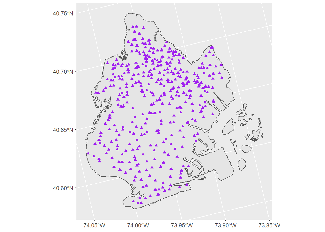
That’s a lot of schools! Before we go any further, let’s try using filter to select only a certain subset of schools.
For instance, maybe we are only interested in high schools. In the school data we can see that there is a variable
that has this information named SCH_TYPE. Using the table command we can look at all the unique types of schools.
# use table() to look at all the unique school types
table(schools$SCH_TYPE)
##
## Early Childhood Elementary High school
## 7 204 119
## Junior High-Intermediate-Middle K-12 all grades K-8
## 92 21 61
## Secondary School
## 33So we see there are 199 high schools. Let’s create a new variable named school_hs which will reflect only the location
of high schools in Brooklyn.
# Filter only high schools
school_hs <- filter(schools, SCH_TYPE == "High school")
And now let’s plot the result with a descriptive title:
# Plot high schools in Brooklyn
ggplot() +
  geom_sf(data = brooklyn) +
  geom_sf(data = school_hs, shape = 17, color = "purple") +
  labs(title = "High Schools in Brooklyn")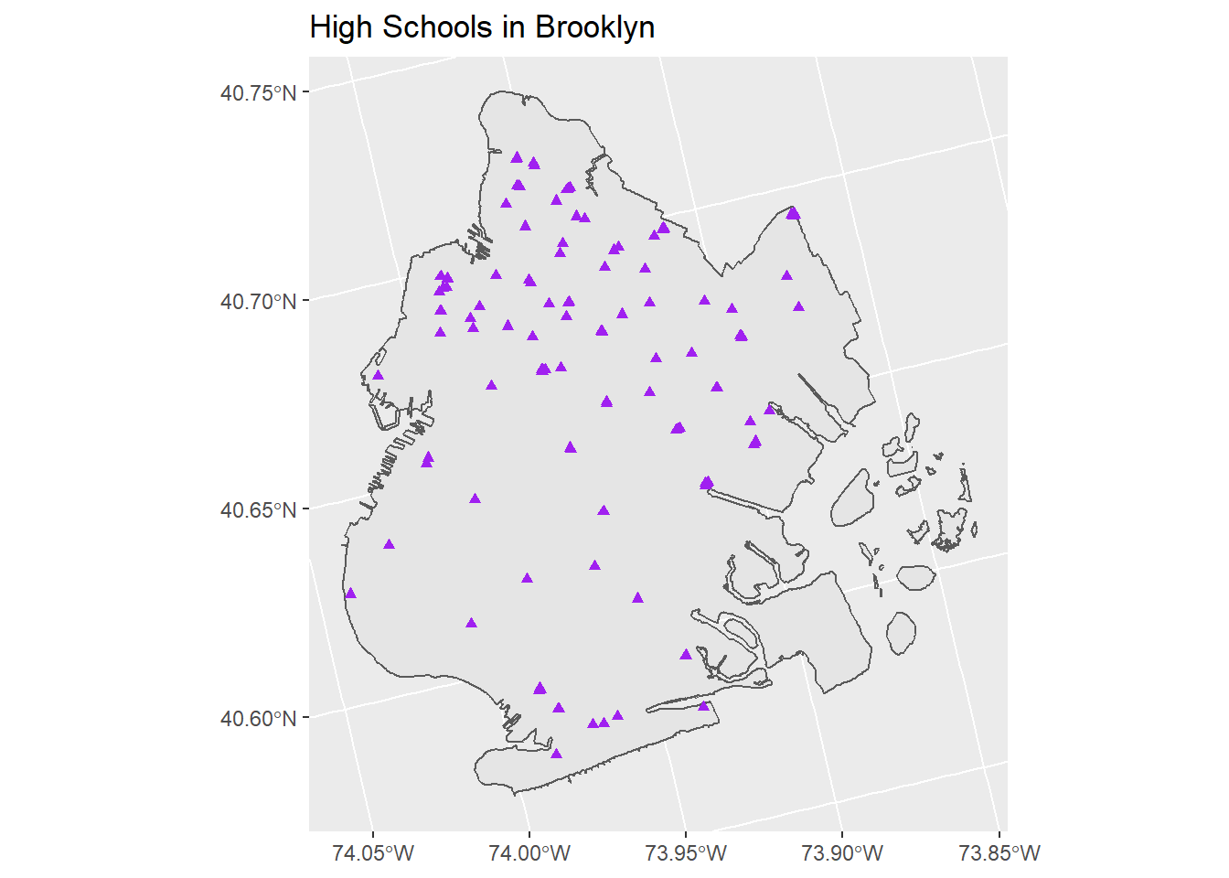
7.1.2 Creating a buffer
Let’s imagine that the mayor of New York wants to know how many robberies have occurred within 1500 feet of high schools
in Brooklyn. As an analyst, we should consider using a buffer to identify the number of incidents in and around
high schools. Let’s introduce a new function: st_buffer. If we do help(st_buffer).
we can get some information about the function:
st_buffer computes a buffer around this geometry/each geometry
This is actually a very simple function which draws a circle of a size of your choice around each individual feature.
So st_buffer here would draw a circle around each school, with a radius of \(n\) feet or meters. Using a bit of math, we
will see that if we set a buffer of a radius of 1500 feet, the diameter of the circle will be \(2r\),
or 2000 feet from end-to-end.
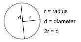
Figure 7.1: Radius and diameter of a circle
Let’s create our buffer. Since a circle is a shape, this process will create a new polygon shapefile, representing a 1500 foot buffer around each school. Also, since our data is projected in meters (rather than feet) we need to do a rough conversion of meters to feet. One meter is about 3.28 feet so: 1500 feet would be:
\[1500/3.28 = 457.3\]
Below, we call the function st_buffer then first provide the shapefile we want to draw buffers around (school),
then specify the distance (in meters) that we want the radius of the buffer to be (dist = 457.3).
This then creates a new shapefile which we can plot.
# Create a buffer, keeping in mind that the data is in METERS
# 457.3 meters = 1500 feet
school_buffer <- st_buffer(school_hs, dist = 457.3)
Let’s try plotting this onto our previous map:
# Plotting school_buffer with fill = NA
# So the buffers aren't colored in
ggplot() +
  geom_sf(data = brooklyn) +
  geom_sf(data = school_hs, shape = 17, color = "purple") +
  geom_sf(data = school_buffer, color = "purple", fill = NA) +
  labs(title = "High Schools in Brooklyn, 1,500 foot buffer")
7.2 Counting Crimes with Spatial Clip and Joins
In our imaginary scenario, let’s imagine we want to find out how many robberies occurred in May within 1,500 of a high
school in Brooklyn. We already have the buffer created, so next we need to get only robberies that occurred in may. If
we look at our crimes dataframe we will see:
# Look at crime data
glimpse(crimes)
## Rows: 19,516
## Columns: 8
## $ CMPLNT_ <int> 179038720, 219802650, 806335079, 619086706, 850815514, 935185889, 267107645, 606415431, 516479438, 376306009~
## $ DATE <date> 2017-12-14, 2017-12-12, 2017-12-24, 2017-12-23, 2017-12-23, 2017-12-12, 2017-12-04, 2017-11-28, 2017-11-24,~
## $ OFNS_DE <chr> "FELONY ASSAULT", "FELONY ASSAULT", "FELONY ASSAULT", "ROBBERY", "BURGLARY", "BURGLARY", "BURGLARY", "ROBBER~
## $ PD_DESC <chr> "STRANGULATION 1ST", "ASSAULT 2,1,UNCLASSIFIED", "STRANGULATION 1ST", "ROBBERY,PERSONAL ELECTRONIC DEVICE", ~
## $ LOC_OF_ <chr> "INSIDE", "FRONT OF", "INSIDE", NA, "INSIDE", "INSIDE", "INSIDE", NA, "INSIDE", "INSIDE", "FRONT OF", "INSID~
## $ PREM_TY <chr> "RESIDENCE - PUBLIC HOUSING", "BAR/NIGHT CLUB", "RESIDENCE - APT. HOUSE", "STREET", "RESIDENCE - APT. HOUSE"~
## $ BORO_NM <chr> "BROOKLYN", "BROOKLYN", "BROOKLYN", "BROOKLYN", "BROOKLYN", "BROOKLYN", "BROOKLYN", "BROOKLYN", "BROOKLYN", ~
## $ geometry <POINT [m]> POINT (1828591 569487.9), POINT (1833544 560962), POINT (1832221 571366.3), POINT (1831581 569645), PO~So we have a little less than 20,000 crime incidents. There is a variable called DATE which records the date of the
crime and a variable called OFNS_DE which is the offense description of the crime. We can use table on this variable
to see how many of each we have.
table(crimes$OFNS_DE)##
## BURGLARY DANGEROUS DRUGS FELONY ASSAULT ROBBERY
## 3742 6039 5600 4135This tells us we have 4 crime types in this dataframe, and the one we want to focus on is robberies. First, let’s start
by applying a filter to the crimes dataframe and pulling out just the data we need. We can use the month function
from lubridate to get just crimes in May by doing month(DATE) == 5 and OFNS_DE == "ROBBERY" will give us just the
robberies.
# Filter the crimes dataframe
# robberies in May
robberies_may <- filter(crimes,
                        month(DATE) == 5,
                        OFNS_DE == "ROBBERY")
If we plot the result on top of our buffers from above, we will get the following map:
# Plot robberies and buffers
ggplot() +
  geom_sf(data = brooklyn) +
  geom_sf(data = robberies_may, size = .6) +
  geom_sf(data = school_buffer, color = "purple", fill = NA) +
  labs(title = "High Schools in Brooklyn, 1,500 foot buffer")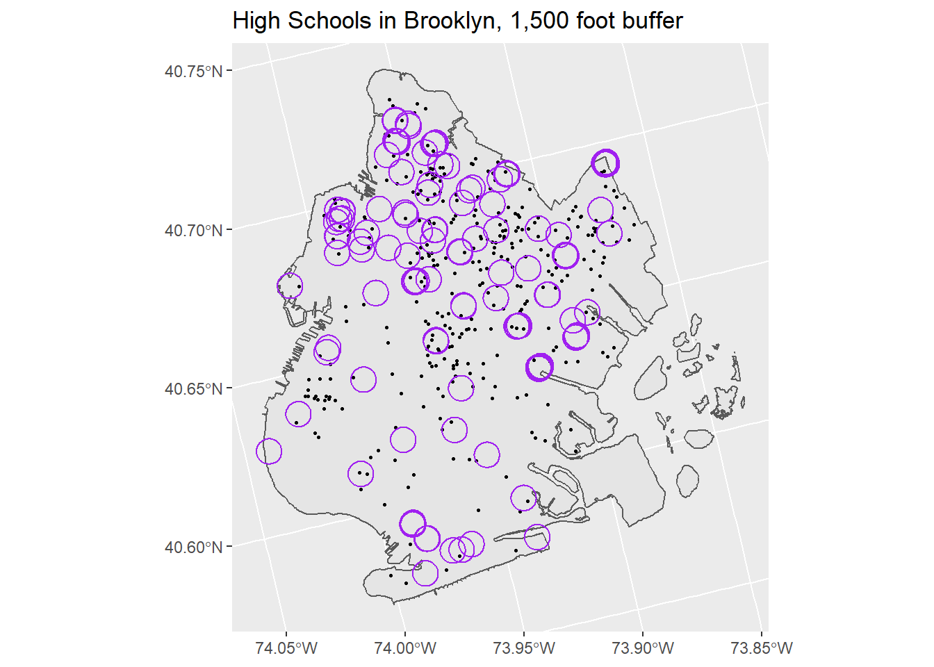
7.2.1 Spatial clip
So we see that some robberies do occur within 1,500 of a school, but many don’t. Let’s start by employing a spatial clip to get only the robberies within the buffer of a school. If you recall, a spatial clip will give us just the features that overlap with another feature (here, robberies that overlap with our buffer).
# Spatial clip to remove only the crimes within the buffer
school_robbery <- robberies_may[school_buffer,]
Now, if we plot this, we will see that we have restricted our view to only the crimes within the buffers.
# Plot robberies and buffers
ggplot() +
  geom_sf(data = brooklyn) +
  geom_sf(data = school_robbery, size = .6) +
  geom_sf(data = school_buffer, color = "purple", fill = NA) +
  labs(title = "High Schools in Brooklyn, 1,500 foot buffer")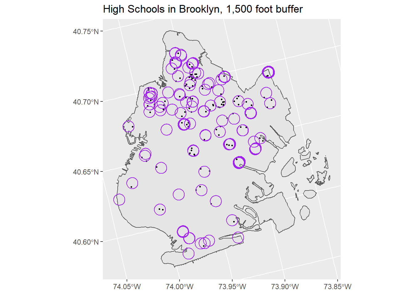
7.2.2 Spatial join
In our second step, we want to find out how many robberies occurred in or around each school. To do this, we need to
spatially join the crimes to the buffer they are within.To do that we are going to need to employ a spatial join. In sf
the command to do this is called st_join. This links two sources of data together based on their shared geometry.
In this case, it will find the crimes that are within the boundaries of all the school buffer zones.
# Use st_join to find crimes within buffers
school_robbery <- st_join(school_robbery, school_buffer)
If we use glimpse on the result of this, we will see that each robbery incident is linked to a school. Now we have
a dataframe with both information on the robbery and the school whose buffer it overlapped with.
glimpse(school_robbery)## Rows: 237
## Columns: 25
## $ CMPLNT_ <int> 441522995, 441522995, 704934966, 149651976, 490020577, 490020577, 490020577, 588172517, 349246259, 1585306~
## $ DATE <date> 2017-05-25, 2017-05-25, 2017-05-14, 2017-05-17, 2017-05-28, 2017-05-28, 2017-05-28, 2017-05-28, 2017-05-2~
## $ OFNS_DE <chr> "ROBBERY", "ROBBERY", "ROBBERY", "ROBBERY", "ROBBERY", "ROBBERY", "ROBBERY", "ROBBERY", "ROBBERY", "ROBBER~
## $ PD_DESC <chr> "ROBBERY,OPEN AREA UNCLASSIFIED", "ROBBERY,OPEN AREA UNCLASSIFIED", "ROBBERY,PERSONAL ELECTRONIC DEVICE", ~
## $ LOC_OF_ <chr> NA, NA, NA, "FRONT OF", "INSIDE", "INSIDE", "INSIDE", "FRONT OF", NA, NA, NA, NA, "FRONT OF", "INSIDE", "I~
## $ PREM_TY <chr> "STREET", "STREET", "STREET", "RESIDENCE - PUBLIC HOUSING", "RESIDENCE - APT. HOUSE", "RESIDENCE - APT. HO~
## $ BORO_NM <chr> "BROOKLYN", "BROOKLYN", "BROOKLYN", "BROOKLYN", "BROOKLYN", "BROOKLYN", "BROOKLYN", "BROOKLYN", "BROOKLYN"~
## $ ATS_CODE <chr> "32K545 ", "32K556 ", "84K473", "14K449 ", "17K408 ", "17K537 ", "17K539 ", ~
## $ BORO <chr> "K", "K", "K", "K", "K", "K", "K", "K", "K", "K", "K", "K", "K", "K", "K", "K", "K", "K", "K", "K", "K", "~
## $ BORONUM <dbl> 2, 2, 2, 2, 2, 2, 2, 2, 2, 2, 2, 2, 2, 2, 2, 2, 2, 2, 2, 2, 2, 2, 3, 3, 2, 2, 2, 2, 2, 2, 2, 2, 2, 2, 2, 2~
## $ LOC_CODE <chr> "K545", "K556", "K473", "K449", "K408", "K537", "K539", "K455", "K594", "K430", "K530", "K646", "K499", "K~
## $ SCHOOLNAME <chr> "EBC HIGH SCHOOL FOR PUBLIC SERVICE\u0096BUSHWICK", "BUSHWICK LEADERS HIGH SCHOOL FOR ACADEMIC EXCELLEN", ~
## $ SCH_TYPE <chr> "High school", "High school", "High school", "High school", "High school", "High school", "High school", "~
## $ MANAGED_BY <dbl> 1, 1, 2, 1, 1, 1, 1, 1, 1, 1, 1, 1, 1, 1, 1, 1, 1, 1, 1, 1, 1, 1, 1, 1, 1, 1, 1, 1, 1, 1, 1, 1, 2, 1, 1, 1~
## $ GEO_DISTRI <dbl> 32, 32, 14, 14, 17, 17, 17, 16, 16, 13, 15, 23, 13, 14, 14, 14, 14, 14, 14, 16, 16, 17, 17, 17, 14, 19, 17~
## $ ADMIN_DIST <dbl> 32, 32, 84, 14, 17, 17, 17, 16, 16, 13, 15, 23, 13, 14, 14, 14, 14, 14, 75, 16, 16, 17, 17, 17, 14, 19, 17~
## $ ADDRESS <chr> "1155 DEKALB AVENUE", "797 BUSHWICK AVENUE", "198 VARET STREET", "325 BUSHWICK AVENUE", "911 FLATBUSH AVEN~
## $ STATE_CODE <chr> "NY", "NY", "NY", "NY", "NY", "NY", "NY", "NY", "NY", "NY", "NY", "NY", "NY", "NY", "NY", "NY", "NY", "NY"~
## $ ZIP <dbl> 11221, 11221, 11206, 11206, 11226, 11226, 11226, 11213, 11233, 11217, 11217, 11233, 11238, 11206, 11211, 1~
## $ PRINCIPAL <chr> "BARNABY SPRING", "CATHERINE REILLY", "Marsha Spampinato", "JASON GRIFFITHS", "ADAM BREIER", "MARY PRENDER~
## $ PRIN_PH <chr> "718-452-3440", "718-919-4212", "718-782-9830", "718-366-0154", "718-564-2580", "718-564-2470", "718-564-2~
## $ FAX <chr> "718-452-3603", "718-574-1103", "347-464-7604", "718-381-3012", "718-564-2581", "718-564-2471", "718-564-2~
## $ GRADES <chr> "09,10,11,12,SE", "09,10,11,12,SE", "09,10,11,12", "09,10,11,12", "09,10,11,12,SE", "09,10,11,12,SE", "09,~
## $ boro_name <chr> "BROOKLYN", "BROOKLYN", "BROOKLYN", "BROOKLYN", "BROOKLYN", "BROOKLYN", "BROOKLYN", "BROOKLYN", "BROOKLYN"~
## $ geometry <POINT [m]> POINT (1833326 571591.3), POINT (1833326 571591.3), POINT (1832318 573135), POINT (1831976 572323.8)~7.2.3 Counting crimes
Now that we have linked robberies to the school buffers we can now count up how many crimes happened at each school
using the count command. There is a variable called SCHOOLNAME which is the identifier for each individual school.
Since we have linked robberies and schools together, we just need to count up how many times each robbery happened near
each school.
# Count up how many crimes happened, for each school
# using `SCHOOLNAME` to count
school_robbery_count <- count(school_robbery, SCHOOLNAME)
That’s it! Now let’s take a look. The count command just creates a new variable named n which is the number of
crimes within 1500 feet of each school. We can do summary to get the summary statistics for this new variable.
summary(school_robbery_count$n)## Min. 1st Qu. Median Mean 3rd Qu. Max.
## 1.000 1.000 2.000 2.347 3.000 10.000Or we can use the command arrange to sort the schools in descending order from highest to lowest. We can see which
school(s) have the most or fewest robberies. In this case ‘P.S. 373 - BROOKLYN TRANSITION CENTER’
had 10 robberies within 1500 feet of the school in May.
arrange(school_robbery_count, desc(n))## Simple feature collection with 101 features and 2 fields
## Geometry type: GEOMETRY
## Dimension: XY
## Bounding box: xmin: 1826759 ymin: 558546.6 xmax: 1838371 ymax: 574362.3
## Projected CRS: Albers
## First 10 features:
## SCHOOLNAME n geometry
## 1 P.S. 373 - BROOKLYN TRANSITION CENTER 10 MULTIPOINT ((1831269 571807...
## 2 GOTHAM PROFESSIONAL ARTS ACADEMY 8 MULTIPOINT ((1833856 569950...
## 3 BROOKLYN LATIN SCHOOL, THE 7 MULTIPOINT ((1831624 572616...
## 4 ACADEMY OF HOSPITALITY AND TOURISM 6 MULTIPOINT ((1831506 566063...
## 5 HIGH SCHOOL FOR SERVICE & LEARNING AT ERASMUS 6 MULTIPOINT ((1831506 566063...
## 6 HIGH SCHOOL FOR YOUTH AND COMMUNITY DEVELOPMENT AT 6 MULTIPOINT ((1831506 566063...
## 7 BROOKLYN ACADEMY OF SCIENCE AND THE ENVIRONMENT 5 MULTIPOINT ((1830901 568673...
## 8 BROOKLYN SCHOOL FOR MUSIC & THEATRE 5 MULTIPOINT ((1830901 568673...
## 9 CLARA BARTON HIGH SCHOOL 5 MULTIPOINT ((1830901 568673...
## 10 FOUNDATIONS ACADEMY 5 MULTIPOINT ((1831161 571699...7.3 Lab 5 Assignment
This lab assignment is worth 10 points. Follow the instructions below.
Using the provided shapefiles crimes_brooklyn.shp, school_brooklyn.shp, and brooklyn.shp
perform the following analyses:
- Filter the
crimes_brooklynfile, based on one of the following crimes, selecting one (or more) months:FELONY ASSAULTBURGLARYDANGEROUS DRUGS
- Filter the
schoolsfile to select a single type of school- Draw a buffer of any size around those schools
- Plot the following in Map 1:
- Your selected crime data (from part 1)
- Your school buffers (from part 2)
- Use a spatial join to count the number of crimes at each school
- Report the summary statistics from crimes within the school buffer
- Identify which school or schools have the most crimes
In your write-up, discuss the crime and type of school you chose in steps 1 and 2. Discuss the buffer size you chose and why you think that size is relevant or applicable to the question at hand. Finally, discuss how many crimes occurred within your buffer and speculate on ways to reduce crime. Answer in at least one to two paragraphs.