Chapter 9 Lab 7 - Clustering
Welcome to Lab 7! In this lab we are going to focus on:
Topics Covered
- Hot Spot Mapping
- Clustering Methods
- Developing Patrol Areas
9.1 Homicides in New Haven
9.1.1 Describing the Problem
Between 2010 and 2019 there were approximately 161 homicides in New Haven. With a population of around 130,000 that averages to a rate of about 12.4 per 100,000. As we can see in the table below, while homicides largely declined from their peak in 2011, they still place New Haven above the national average.
| year | Homicides | Rate |
|---|---|---|
| 2010 | 23 | 17.69 |
| 2011 | 34 | 26.15 |
| 2012 | 14 | 10.77 |
| 2013 | 20 | 15.38 |
| 2014 | 13 | 10.00 |
| 2015 | 15 | 11.54 |
| 2016 | 13 | 10.00 |
| 2017 | 7 | 5.38 |
| 2018 | 10 | 7.69 |
| 2019 | 12 | 9.23 |
Imagine the city of New Haven wants to implement a strategic plan to reduce homicide in the city’s hardest-hit neighborhoods. Of course, the city doesn’t have unlimited money, so you need to identify a subset of areas that have historically experienced the most homicides. After identifying these locations, you can then move to community-based outreach and support to help lessen the effects of violent crime. So where do we start?
9.1.2 Setting up the Data
Before we do anything else, let’s start by loading in our data, all of our tools, and creating a quick point map of the
crime data. For this lab we will need both the kernel_density tool, as well as the new cluster_points tool. We can
load them the same way we have done in previous lab assignments.
library(sf)
library(tidyverse)

load("C:/Users/gioc4/Desktop/cluster_points.Rdata")
load("C:/Users/gioc4/Desktop/kernel_density.Rdata")

new_haven <- st_read("C:/Users/gioc4/Desktop/nh_blocks.shp")
homicide <- st_read("C:/Users/gioc4/Desktop/nh_homicides.shp")
Now that we have everything loaded in, let’s create a point map using both our shapefiles. We’ll keep it simple and display the New Haven homicides as simple red points.
# Plot point map of new haven homicides
ggplot() +
  geom_sf(data = new_haven) +
  geom_sf(data = homicide, color = 'red')
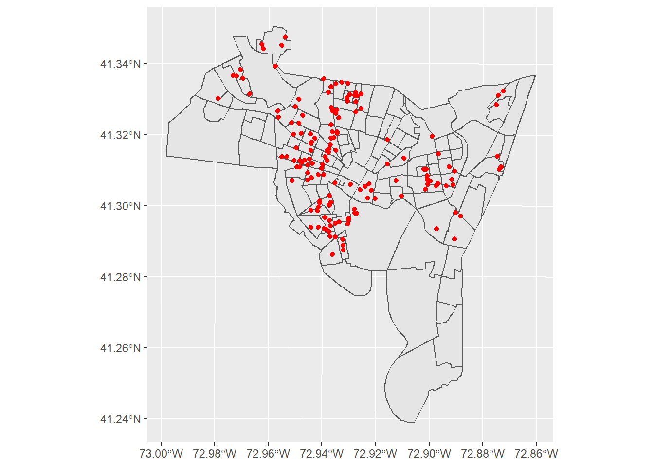
This point map helps: we can see historically homicides have largely occurred on the West-central part of the city, with a few other clusters in the South and East. However, since we have so many overlapping points it is difficult to discern exactly where we might want to focus our community initiative. That is a common problem we have run into in the past. While we have a number of options for identifying clusters of points, let’s begin with one we are familiar with: hot spot mapping.
9.2 Hot Spot Mapping
Let’s create a quick hot spot map using the kernel_density function. If you recall, we used this same method in
Lab 3 to create hot spots of burglaries and breaches of the peace. Here, let’s do a quick hot spot map by
setting the bandwidth to 1,500 feet. We won’t plot the quick plot by setting plot = FALSE and just add the data
directly to ggplot.
# Calculate the kernel density estimate w/o plotting
newhaven_kde <- kernel_density(homicide, new_haven, bdw = 1500, plot = FALSE)

# Plot the results in ggplot
ggplot() +
  geom_sf(data = new_haven, fill = NA, size = 1, color = "black") +
  geom_raster(data = newhaven_kde, aes(x = X, y = Y, fill = density)) +
  scale_fill_viridis_c(option = "plasma") +
  theme_void()
This hot spot map confirms mostly what we saw in the point map - namely that there are a few clusters in the Central-West and East part of the city. Hot spot maps can be very useful - but sometimes we might want to come up with a method that has more defined borders. Imagine we wanted to be able to draw a rough circle around a few hotspots and focus our attention on those areas. How might we do that?
9.3 Clustering
Hot spot mapping using kernel density estimation is a method of estimating the overal density of points in an area. However, sometimes we want to identify clusters of similar points and group them together. This is a type of classification problem that is often known as unsupervised learning in data science. The specific method we will apply here is known as a DBscan or a Density-based spatial clustering of applications with noise.
9.3.1 DBscan
We will be making use of a new function called dbscan. To begin, we should install the package we will need.
# install dbscan package
install.packages("dbscan")
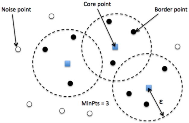
The DBscan method is a type of point clustering which helps identify clusters of similar points based on their location, while ignoring points that are likely random (referred to here as ‘noise’). The idea is that we can provide the computer with some guidelines, and then it will try and find as many point clusters that fit those guidelines. Looking at the image below, we can see how the DBscan method identifies overlapping areas of distance based on a ‘core’ point, and then clusters other points around those together. \(\epsilon\) in the image below refers to the maximum distance around a core point.

Figure 9.1: DBscan clustering
To do this in R we’re going to use another custom function called cluster_points. Just like the kernel_density
function, the cluster_points function only requires a minimum of two things:
point_data: The points you want to clusterpolygon_data: The polygon shapefile of the region
However, we will also want to provide some rules about what we would consider a cluster. To do this we also need to add:
pts: The minimum number of points for a clusterdist: The maximum distance of points for a cluster
So for #3, this is just how many points we would consider reasonable to be a cluster. In this case, given the relative infrequency of homicide, we might say that 5 points is the minimum number we would consider to be a cluster. In addition we need to think about the maximum distance these points should be from each other to still be a cluster. Just like with kernel density mapping, too big a number will cluster almost everything, while too small a number will make finding reasonable clusters hard. Let’s start with our number here and see what happens:
# Find clusters with:
# at least 5 points
# within 1000 feet of each other
cluster_points(homicide, new_haven, pts = 5, dist = 1000)
## DBSCAN clustering for 161 objects.
## Parameters: eps = 1000, minPts = 5
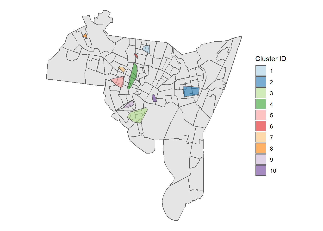
## The clustering contains 10 cluster(s) and 53 noise points.
##
## 0 1 2 3 4 5 6 7 8 9 10
## 53 9 17 21 19 12 6 5 5 9 5
##
## Available fields: cluster, eps, minPts
Based on the metrics provided in our code, we see that the program identified 10 total clusters - some of which with only 5 or 6 points, while some have upwards of 20. For example, we see that cluster 3 is the largest with 21 total homicides (the light-green area in the bottom-left of the map). While this is helpful, we might want to focus on larger, more geographically contiguous areas. We can adjust our DBscan search and see what we come up with.
Let’s try restricting our search by changing the pts and dist parameters. Let’s say we want to try and find clusters
that comprise more homicides, as well as encompassing a larger area. We can accomplish that by increasing pts to 10
and dist to 1500. So, now we will find larger clusters which have more points. Let’s see what that looks like:
# Find clusters with:
# at least 10 points
# within 1500 feet of each other
cluster_points(homicide, new_haven, pts = 10, dist = 1500)
## DBSCAN clustering for 161 objects.
## Parameters: eps = 1500, minPts = 10
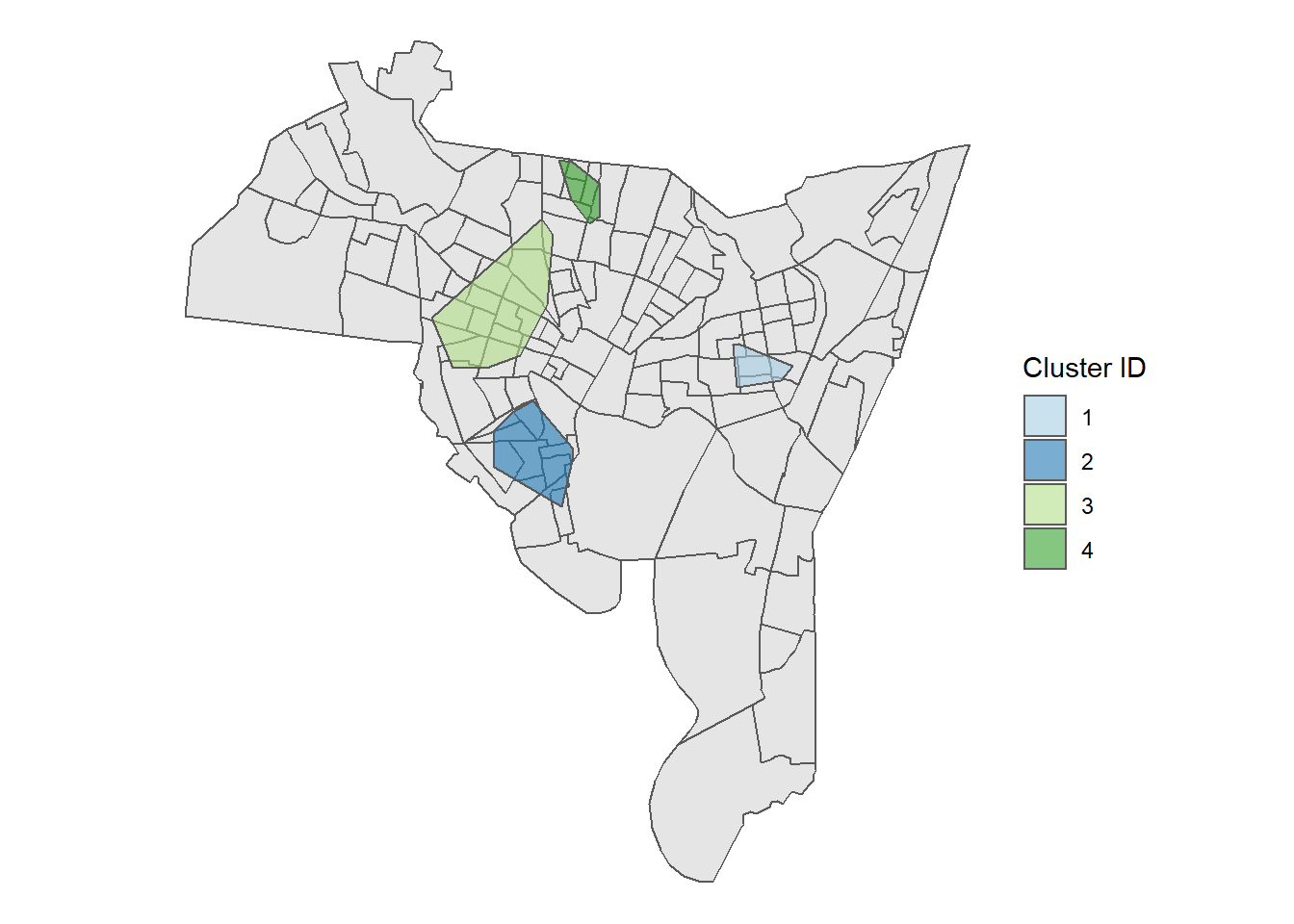
## The clustering contains 4 cluster(s) and 66 noise points.
##
## 0 1 2 3 4
## 66 14 29 40 12
##
## Available fields: cluster, eps, minPts
So, based on the output we have 4 total clusters. Cluster 1 and 4 are relatively small, while clusters 2 and 3 are much larger. Cluster 3 in particular has 40 homicides, which is about 25% of all homicides in New Haven. Given our limited resources, we might focus on the neighborhood around Cluster 3.
We can also identify how big an area these clusters cover, and how many incidents they encompass. To do this, all
we have to do is add an additional argument to the function that says print_area = TRUE.
# Setting 'print_area' to TRUE
cluster_points(homicide, new_haven, pts = 10, dist = 1500, print_area = TRUE)
## DBSCAN clustering for 161 objects.
## Parameters: eps = 1500, minPts = 10
## The clustering contains 4 cluster(s) and 66 noise points.
##
## 0 1 2 3 4
## 66 14 29 40 12
##
## Available fields: cluster, eps, minPts
## [1] "Proportion of Area: 0.07"
## [1] "Proportion of Incidents: 0.61"
So this tells us that our 4 clusters make up about 7% of the city and capture about 61% of all homicides.
9.4 Lab 7 Assignment
This lab assignment is worth 10 points. Follow the instructions below.
Use either the nh_breach.shp or nh_burg.shp files to do the following analyses:
- Create either a point map or a hot spot map displaying the patterns of crime across New Haven
- Be sure to use custom colors, shapes, sizes, or patterns
- Add a title to your plot
- Using the crime you chose from step 1, use the
cluster_pointsfunction to identify clusters- Specify both the
ptsanddistfunction - Provide a reasonable description of why you chose those values
- Specify both the
In your write up, discuss the patterns you observed in step 1 and how they were similar or different from what you observed in step 2. Describe how you would organize a crime prevention strategy based on these patterns, and whether they would be tactical or strategic.