Chapter 10 Reordering to match datasets
10.1 Reordering data to match
In the previous lesson, we learned how to determine whether the same data is present in two datasets, in addition to, whether it is in the same order. In this lesson, we will explore how to reorder the data such that the datasets are matching.
Exercise
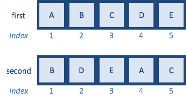
Now that we know how to reorder using indices, let’s try to use it to reorder the contents of one vector to match the contents of another. Let’s create the vectors first and second as detailed below:

How would you reorder the second vector to match first?
If we had large datasets, it would be difficult to reorder them by searching for the indices of the matching elements, and it would be quite easy to make a typo or mistake. To help with matching datasets, there is a function called match().
10.2 The match function
We can use the match() function to match the values in two vectors. We’ll be using it to evaluate which values are present in both vectors, and how to reorder the elements to make the values match.
match() takes 2 arguments. The first argument is a vector of values in the order you want, while the second argument is the vector of values to be reordered such that it will match the first:
- a vector of values in the order you want
- a vector of values to be reordered
The function returns the position of the matches (indices) with respect to the second vector, which can be used to re-order it so that it matches the order in the first vector. Let’s use match() on the first and second vectors we created.
The output is the indices for how to reorder the second vector to match the first. These indices match the indices that we derived manually before.
Now, we can just use the indices to reorder the elements of the second vector to be in the same positions as the matching elements in the first vector:
Then, we can use those indices to reorder the second vector similar to how we ordered with the manually derived indices.
If the output looks good, we can save the reordered vector to a new variable.

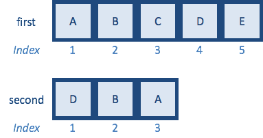
Now that we know how match() works, let’s change vector second so that only a subset are retained:

And try to match() again:
We see that the match() function takes every element in the first vector and finds the position of that element in the second vector, and if that element is not present, will return a missing value of NA. The value NA represents missing data for any data type within R. In this case, we can see that the match() function output represents the value at position 3 as first, which is A, then position 2 is next, which is B, the value coming next is supposed to be C, but it is not present in the second vector, so NA is returned, so on and so forth.
NOTE: For values that don’t match by default return an
NAvalue. You can specify what values you would have it assigned usingnomatchargument. Also, if there is more than one matching value found only the first is reported.
If we rearrange second using these indices, then we should see that all the values present in both vectors are in the same positions and NAs are present for any missing values.
Reordering genomic data using match() function
While the input to the match() function is always going to be to vectors, often we need to use these vectors to reorder the rows or columns of a data frame to match the rows or columns of another dataframe. Let’s explore how to do this with our use case featuring RNA-seq data. To perform differential gene expression analysis, we have a data frame with the expression data or counts for every sample and another data frame with the information about to which condition each sample belongs. For the tools doing the analysis, the samples in the counts data, which are the column names, need to be the same and in the same order as the samples in the metadata data frame, which are the rownames.
We can take a look at these samples in each dataset by using the rownames() and colnames() functions.
# Check row names of the metadata
rownames(metadata)

# Check the column names of the counts data
colnames(rpkm_data)
We see the row names of the metadata are in a nice order starting at sample1 and ending at sample12, while the column names of the counts data look to be the same samples, but are randomly ordered. Therefore, we want to reorder the columns of the counts data to match the order of the row names of the metadata. To do so, we will use the match() function to match the row names of our metadata with the column names of our counts data, so these will be the arguments for match.
To do so, we will use the match function to match the row names of our metadata with the column names of our counts data, so these will be the arguments for match().
Within the match() function, the rownames of the metadata is the vector in the order that we want, so this will be the first argument, while the column names of the count or rpkm data is the vector to be reordered. We will save these indices for how to reorder the column names of the count data such that it matches the rownames of the metadata to a variable called genomic idx.
The genomic_idx represents how to re-order the column names in our counts data to be identical to the row names in metadata.
Now we can create a new counts data frame in which the columns are re-ordered based on the match() indices. Remember that to reorder the rows or columns in a data frame we give the name of the data frame followed by square brackets, and then the indices for how to reorder the rows or columns.
Our genomic_idx represents how we would need to reorder the columns of our count data such that the column names would be in the same order as the row names of our metadata. Therefore, we need to add our genomic_idx to the columns position. We are going to save the output of the reordering to a new data frame called rpkm_ordered.
# Reorder the counts data frame to have the sample names in the same order as the metadata data frame
rpkm_ordered  <- rpkm_data[ , genomic_idx]
Check and see what happened by clicking on the rpkm_ordered in the Environment window or using the View() function.
We can see the sample names are now in a nice order from sample 1 to 12, just like the metadata.
You can also verify that column names of this new data matrix matches the metadata row names by using the all function:
Now that our samples are ordered the same in our metadata and counts data, if these were raw counts (not RPKM) we could proceed to perform differential expression analysis with this dataset.
Exercises
After talking with your collaborator, it becomes clear that
sample2andsample9were actually from a different mouse background than the other samples and should not be part of our analysis. Create a new variable calledsubset_rpkmthat has these columns removed from therpkm_ordereddata frame.Use the
match()function to subset themetadatadata frame so that the row names of themetadatadata frame match the column names of thesubset_rpkmdata frame.