Chapter 17 Codebook for IntroR and RStudio
69 points total
17.1 01 Setting up R and RStudio
Let’s start by going to the environment panel in RStudio and clearing the environment. This is a good habit to get into when starting a new project, as it ensures that you are starting with a clean slate.
17.2 02 Introduction to R and RStudio
.md file = 02-introR-R-and-RStudio.md
17.2.1 Running commands and annotating code:
Add some additional code to the following chunk:
## [1] 8The chunk will run inline and output inline, but I prefer to set the chunk so it will run in the console, because it gives us extra room, especially for plotting. You can set this using the cog wheel at the top of the script window next to the Knit button.
17.2.2 The assignment operator (<-)
The assignment operator assigns values on the right to variables on the left.
In RStudio the keyboard shortcut for the assignment operator <- is Alt + - (Windows) or Option + - (Mac).
## [1] 8## [1] 8Exercise points +2
- Try changing the value of the variable x to 5. What happens to number?
- Ans:
- Now try changing the value of variable y to contain the value 10. What do you need to do, to update the variable number?
- Ans:
17.3 03 R syntax and data structures
.md file = 03-introR-syntax-and-data-structures.md
17.3.1 Vectors
# Create a numeric vector and store the vector as a variable called 'glengths'
glengths <- c(4.6, 3000, 50000)
glengths
## [1] 4.6 3000.0 50000.0# Create a character vector and store the vector as a variable called 'species'
species <- c("ecoli", "human", "corn")
species## [1] "ecoli" "human" "corn"Exercise points +1
Try to create a vector of numeric and character values by combining the two vectors that we just created (glengths and species). Assign this combined vector to a new variable called combined. Hint: you will need to use the combine c() function to do this. Print the combined vector in the console, what looks different compared to the original vectors?
- Ans:
17.3.2 Factors
Create a character vector and store the vector as a variable called ‘expression’
## [1] "low" "high" "medium" "high" "low" "medium" "high"Turn ‘expression’ vector into a factor
## [1] low high medium high low medium high
## Levels: high low medium## [1] 7## [1] "high" "low" "medium"Exercises points +2
Let’s say that in our experimental analyses, we are working with three different sets of cells: normal, cells knocked out for geneA (a very exciting gene), and cells overexpressing geneA. We have three replicates for each celltype.
- Create a vector named samplegroup with nine elements: 3 control (“CTL”) values, 3 knock-out (“KO”) values, and 3 over-expressing (“OE”) values.
- Turn samplegroup into a factor data structure.
17.3.3 Dataframes
A data.frame is the de facto data structure for most tabular data and what we use for statistics and plotting. A data.frame is similar to a matrix in that it’s a collection of vectors of the same length and each vector represents a column. However, in a dataframe each vector can be of a different data type (e.g., characters, integers, factors). A dataframe can be created using the data.frame() function.
## species glengths
## 1 ecoli 4.6
## 2 human 3000.0
## 3 corn 50000.0Exercise points +1
Create a data frame called favorite_books with the following vectors as columns:
17.4 04 Functions in R
.md file = 04-introR-functions-and-arguments.md
17.4.1 Basic functions
We have already used a few examples of basic functions in the previous lessons i.e c(), and factor().
Many of the base functions in R involve mathematical operations. One example would be the function sqrt(). The input/argument must be a number, and the output is the square root of that number. Let’s try finding the square root of 81:
## [1] 9## [1] 2.144761 54.772256 223.606798Round function:
## [1] 3## [1] 3.14You can also round in the opposite direction, for example, to the nearest 100 by setting the digits argument to -2:
## [1] 40017.4.2 Seeking help on functions
## function (x, digits = 0, ...)
## NULL##
## round> round(.5 + -2:4) # IEEE / IEC rounding: -2 0 0 2 2 4 4
## [1] -2 0 0 2 2 4 4
##
## round> ## (this is *good* behaviour -- do *NOT* report it as bug !)
## round>
## round> ( x1 <- seq(-2, 4, by = .5) )
## [1] -2.0 -1.5 -1.0 -0.5 0.0 0.5 1.0 1.5 2.0 2.5 3.0 3.5 4.0
##
## round> round(x1) #-- IEEE / IEC rounding !
## [1] -2 -2 -1 0 0 0 1 2 2 2 3 4 4
##
## round> x1[trunc(x1) != floor(x1)]
## [1] -1.5 -0.5
##
## round> x1[round(x1) != floor(x1 + .5)]
## [1] -1.5 0.5 2.5
##
## round> (non.int <- ceiling(x1) != floor(x1))
## [1] FALSE TRUE FALSE TRUE FALSE TRUE FALSE TRUE FALSE TRUE FALSE TRUE
## [13] FALSE
##
## round> x2 <- pi * 100^(-1:3)
##
## round> round(x2, 3)
## [1] 0.031 3.142 314.159 31415.927 3141592.654
##
## round> signif(x2, 3)
## [1] 3.14e-02 3.14e+00 3.14e+02 3.14e+04 3.14e+06Exercise points +3
- Let’s use base R function to calculate mean value of the
glengthsvector. You might need to search online to find what function can perform this task.
- Create a new vector
test <- c(1, NA, 2, 3, NA, 4). Use the same base R function from exercise 1 (with addition of proper argument), and calculate the mean value of thetestvector. The output should be 2.5.
NOTE: In R, missing values are represented by the symbol
NA(not available).
It’s a way to make sure that users know they have missing data, and make a conscious decision on how to deal with it.
There are ways to ignoreNAduring statistical calculation, or to removeNAfrom the vector.
- Another commonly used base function is sort(). Use this function to sort the
glengthsvector in descending order.
17.4.3 User-defined Functions
Let’s try creating a simple example function. This function will take in a numeric value as input, and return the squared value.
Once you run the code, you should see a function named square_it in the Environment panel (located at the top right of Rstudio interface). Now, we can use this function as any other base R functions. We type out the name of the function, and inside the parentheses we provide a numeric value x:
## [1] 25Pretty simple, right? In this case, we only had one line of code that was run, but in theory you could have many lines of code to get obtain the final results that you want to “return” to the user. We have only scratched the surface here when it comes to creating functions! If you are interested you can also find more detailed information on writing functions R-bloggers site.
Exercise points +2
- Write a function called
multiply_it, which takes two inputs: a numeric valuex, and a numeric valuey. The function will return the product of these two numeric values, which isx * y. For example,multiply_it(x=4, y=6)will return output24.
Function:
Demo:
17.5 05 Packages and libraries
.md file = 05-introR_packages.md
17.5.1 Packages and Libraries
You can check what libraries (packages) are loaded in your current R session by typing into the console:
## R version 4.4.1 (2024-06-14)
## Platform: x86_64-apple-darwin20
## Running under: macOS Sonoma 14.6.1
##
## Matrix products: default
## BLAS: /System/Library/Frameworks/Accelerate.framework/Versions/A/Frameworks/vecLib.framework/Versions/A/libBLAS.dylib
## LAPACK: /Library/Frameworks/R.framework/Versions/4.4-x86_64/Resources/lib/libRlapack.dylib; LAPACK version 3.12.0
##
## locale:
## [1] en_US.UTF-8/en_US.UTF-8/en_US.UTF-8/C/en_US.UTF-8/en_US.UTF-8
##
## time zone: America/Los_Angeles
## tzcode source: internal
##
## attached base packages:
## [1] stats graphics grDevices utils datasets methods base
##
## other attached packages:
## [1] bookdown_0.40 lubridate_1.9.3 forcats_1.0.0 stringr_1.5.1
## [5] dplyr_1.1.4 readr_2.1.5 tidyr_1.3.1 tibble_3.2.1
## [9] tidyverse_2.0.0 gplots_3.1.3.1 purrr_1.0.2 ggplot2_3.5.1
##
## loaded via a namespace (and not attached):
## [1] sass_0.4.9 utf8_1.2.4 generics_0.1.3 bitops_1.0-8
## [5] KernSmooth_2.23-24 gtools_3.9.5 stringi_1.8.4 hms_1.1.3
## [9] digest_0.6.37 magrittr_2.0.3 caTools_1.18.3 timechange_0.3.0
## [13] evaluate_0.24.0 grid_4.4.1 fastmap_1.2.0 jsonlite_1.8.8
## [17] tinytex_0.53 formatR_1.14 fansi_1.0.6 scales_1.3.0
## [21] jquerylib_0.1.4 cli_3.6.3 crayon_1.5.3 rlang_1.1.4
## [25] bit64_4.0.5 munsell_0.5.1 withr_3.0.1 cachem_1.1.0
## [29] yaml_2.3.10 parallel_4.4.1 tools_4.4.1 tzdb_0.4.0
## [33] colorspace_2.1-1 vctrs_0.6.5 R6_2.5.1 lifecycle_1.0.4
## [37] bit_4.0.5 vroom_1.6.5 archive_1.1.9 pkgconfig_2.0.3
## [41] pillar_1.9.0 bslib_0.8.0 gtable_0.3.5 rsconnect_1.3.1
## [45] glue_1.7.0 xfun_0.47 tidyselect_1.2.1 highr_0.11
## [49] rstudioapi_0.16.0 knitr_1.48 farver_2.1.2 htmltools_0.5.8.1
## [53] rmarkdown_2.28 labeling_0.4.3 compiler_4.4.1## [1] ".GlobalEnv" "package:bookdown" "package:lubridate"
## [4] "package:forcats" "package:stringr" "package:dplyr"
## [7] "package:readr" "package:tidyr" "package:tibble"
## [10] "package:tidyverse" "package:gplots" "package:purrr"
## [13] "package:ggplot2" "tools:rstudio" "package:stats"
## [16] "package:graphics" "package:grDevices" "package:utils"
## [19] "package:datasets" "package:methods" "Autoloads"
## [22] "package:base"17.5.2 Installing packages
17.5.2.1 Packages from CRAN:
Previously we have introduced you to installing packages. An example is given below for the ggplot2 package that will be required for some plots we will create later on. Run this code to install ggplot2.
Set eval = TRUE if you haven’t installed ggplot2 yet
Alternatively, packages can also be installed from Bioconductor, a repository of packages which provides tools for the analysis and comprehension of high-throughput genomic data.
Set eval = TRUE if you haven’t installed BiocManager yet
17.5.2.2 Packages from Bioconductor:
Now you can use BiocManager::install to install packages available on Bioconductor. Bioconductor is a free, open source and open development software project for the analysis and comprehension of genomic data generated by wet lab experiments in molecular biology.
17.5.3 Loading libraries/packages
To see the functions in a package you can also type:
## [1] "%+%" "%+replace%"
## [3] "aes" "aes_"
## [5] "aes_all" "aes_auto"
## [7] "aes_q" "aes_string"
## [9] "after_scale" "after_stat"
## [11] "alpha" "annotate"
## [13] "annotation_custom" "annotation_logticks"
## [15] "annotation_map" "annotation_raster"
## [17] "arrow" "as_label"
## [19] "as_labeller" "autolayer"
## [21] "autoplot" "AxisSecondary"
## [23] "benchplot" "binned_scale"
## [25] "borders" "calc_element"
## [27] "check_device" "combine_vars"
## [29] "continuous_scale" "Coord"
## [31] "coord_cartesian" "coord_equal"
## [33] "coord_fixed" "coord_flip"
## [35] "coord_map" "coord_munch"
## [37] "coord_polar" "coord_quickmap"
## [39] "coord_radial" "coord_sf"
## [41] "coord_trans" "CoordCartesian"
## [43] "CoordFixed" "CoordFlip"
## [45] "CoordMap" "CoordPolar"
## [47] "CoordQuickmap" "CoordRadial"
## [49] "CoordSf" "CoordTrans"
## [51] "cut_interval" "cut_number"
## [53] "cut_width" "datetime_scale"
## [55] "derive" "diamonds"
## [57] "discrete_scale" "draw_key_abline"
## [59] "draw_key_blank" "draw_key_boxplot"
## [61] "draw_key_crossbar" "draw_key_dotplot"
## [63] "draw_key_label" "draw_key_linerange"
## [65] "draw_key_path" "draw_key_point"
## [67] "draw_key_pointrange" "draw_key_polygon"
## [69] "draw_key_rect" "draw_key_smooth"
## [71] "draw_key_text" "draw_key_timeseries"
## [73] "draw_key_vline" "draw_key_vpath"
## [75] "dup_axis" "economics"
## [77] "economics_long" "el_def"
## [79] "element_blank" "element_grob"
## [81] "element_line" "element_rect"
## [83] "element_render" "element_text"
## [85] "enexpr" "enexprs"
## [87] "enquo" "enquos"
## [89] "ensym" "ensyms"
## [91] "expand_limits" "expand_scale"
## [93] "expansion" "expr"
## [95] "Facet" "facet_grid"
## [97] "facet_null" "facet_wrap"
## [99] "FacetGrid" "FacetNull"
## [101] "FacetWrap" "faithfuld"
## [103] "fill_alpha" "find_panel"
## [105] "flip_data" "flipped_names"
## [107] "fortify" "Geom"
## [109] "geom_abline" "geom_area"
## [111] "geom_bar" "geom_bin_2d"
## [113] "geom_bin2d" "geom_blank"
## [115] "geom_boxplot" "geom_col"
## [117] "geom_contour" "geom_contour_filled"
## [119] "geom_count" "geom_crossbar"
## [121] "geom_curve" "geom_density"
## [123] "geom_density_2d" "geom_density_2d_filled"
## [125] "geom_density2d" "geom_density2d_filled"
## [127] "geom_dotplot" "geom_errorbar"
## [129] "geom_errorbarh" "geom_freqpoly"
## [131] "geom_function" "geom_hex"
## [133] "geom_histogram" "geom_hline"
## [135] "geom_jitter" "geom_label"
## [137] "geom_line" "geom_linerange"
## [139] "geom_map" "geom_path"
## [141] "geom_point" "geom_pointrange"
## [143] "geom_polygon" "geom_qq"
## [145] "geom_qq_line" "geom_quantile"
## [147] "geom_raster" "geom_rect"
## [149] "geom_ribbon" "geom_rug"
## [151] "geom_segment" "geom_sf"
## [153] "geom_sf_label" "geom_sf_text"
## [155] "geom_smooth" "geom_spoke"
## [157] "geom_step" "geom_text"
## [159] "geom_tile" "geom_violin"
## [161] "geom_vline" "GeomAbline"
## [163] "GeomAnnotationMap" "GeomArea"
## [165] "GeomBar" "GeomBlank"
## [167] "GeomBoxplot" "GeomCol"
## [169] "GeomContour" "GeomContourFilled"
## [171] "GeomCrossbar" "GeomCurve"
## [173] "GeomCustomAnn" "GeomDensity"
## [175] "GeomDensity2d" "GeomDensity2dFilled"
## [177] "GeomDotplot" "GeomErrorbar"
## [179] "GeomErrorbarh" "GeomFunction"
## [181] "GeomHex" "GeomHline"
## [183] "GeomLabel" "GeomLine"
## [185] "GeomLinerange" "GeomLogticks"
## [187] "GeomMap" "GeomPath"
## [189] "GeomPoint" "GeomPointrange"
## [191] "GeomPolygon" "GeomQuantile"
## [193] "GeomRaster" "GeomRasterAnn"
## [195] "GeomRect" "GeomRibbon"
## [197] "GeomRug" "GeomSegment"
## [199] "GeomSf" "GeomSmooth"
## [201] "GeomSpoke" "GeomStep"
## [203] "GeomText" "GeomTile"
## [205] "GeomViolin" "GeomVline"
## [207] "get_alt_text" "get_element_tree"
## [209] "get_guide_data" "gg_dep"
## [211] "ggplot" "ggplot_add"
## [213] "ggplot_build" "ggplot_gtable"
## [215] "ggplotGrob" "ggproto"
## [217] "ggproto_parent" "ggsave"
## [219] "ggtitle" "Guide"
## [221] "guide_axis" "guide_axis_logticks"
## [223] "guide_axis_stack" "guide_axis_theta"
## [225] "guide_bins" "guide_colorbar"
## [227] "guide_colorsteps" "guide_colourbar"
## [229] "guide_coloursteps" "guide_custom"
## [231] "guide_gengrob" "guide_geom"
## [233] "guide_legend" "guide_merge"
## [235] "guide_none" "guide_train"
## [237] "guide_transform" "GuideAxis"
## [239] "GuideAxisLogticks" "GuideAxisStack"
## [241] "GuideAxisTheta" "GuideBins"
## [243] "GuideColourbar" "GuideColoursteps"
## [245] "GuideCustom" "GuideLegend"
## [247] "GuideNone" "GuideOld"
## [249] "guides" "has_flipped_aes"
## [251] "is.Coord" "is.facet"
## [253] "is.ggplot" "is.ggproto"
## [255] "is.theme" "label_both"
## [257] "label_bquote" "label_context"
## [259] "label_parsed" "label_value"
## [261] "label_wrap_gen" "labeller"
## [263] "labs" "last_plot"
## [265] "layer" "layer_data"
## [267] "layer_grob" "layer_scales"
## [269] "layer_sf" "Layout"
## [271] "lims" "luv_colours"
## [273] "map_data" "margin"
## [275] "max_height" "max_width"
## [277] "mean_cl_boot" "mean_cl_normal"
## [279] "mean_sdl" "mean_se"
## [281] "median_hilow" "merge_element"
## [283] "midwest" "mpg"
## [285] "msleep" "new_guide"
## [287] "old_guide" "panel_cols"
## [289] "panel_rows" "pattern_alpha"
## [291] "Position" "position_dodge"
## [293] "position_dodge2" "position_fill"
## [295] "position_identity" "position_jitter"
## [297] "position_jitterdodge" "position_nudge"
## [299] "position_stack" "PositionDodge"
## [301] "PositionDodge2" "PositionFill"
## [303] "PositionIdentity" "PositionJitter"
## [305] "PositionJitterdodge" "PositionNudge"
## [307] "PositionStack" "presidential"
## [309] "qplot" "quickplot"
## [311] "quo" "quo_name"
## [313] "quos" "register_theme_elements"
## [315] "rel" "remove_missing"
## [317] "render_axes" "render_strips"
## [319] "reset_theme_settings" "resolution"
## [321] "Scale" "scale_alpha"
## [323] "scale_alpha_binned" "scale_alpha_continuous"
## [325] "scale_alpha_date" "scale_alpha_datetime"
## [327] "scale_alpha_discrete" "scale_alpha_identity"
## [329] "scale_alpha_manual" "scale_alpha_ordinal"
## [331] "scale_color_binned" "scale_color_brewer"
## [333] "scale_color_continuous" "scale_color_date"
## [335] "scale_color_datetime" "scale_color_discrete"
## [337] "scale_color_distiller" "scale_color_fermenter"
## [339] "scale_color_gradient" "scale_color_gradient2"
## [341] "scale_color_gradientn" "scale_color_grey"
## [343] "scale_color_hue" "scale_color_identity"
## [345] "scale_color_manual" "scale_color_ordinal"
## [347] "scale_color_steps" "scale_color_steps2"
## [349] "scale_color_stepsn" "scale_color_viridis_b"
## [351] "scale_color_viridis_c" "scale_color_viridis_d"
## [353] "scale_colour_binned" "scale_colour_brewer"
## [355] "scale_colour_continuous" "scale_colour_date"
## [357] "scale_colour_datetime" "scale_colour_discrete"
## [359] "scale_colour_distiller" "scale_colour_fermenter"
## [361] "scale_colour_gradient" "scale_colour_gradient2"
## [363] "scale_colour_gradientn" "scale_colour_grey"
## [365] "scale_colour_hue" "scale_colour_identity"
## [367] "scale_colour_manual" "scale_colour_ordinal"
## [369] "scale_colour_steps" "scale_colour_steps2"
## [371] "scale_colour_stepsn" "scale_colour_viridis_b"
## [373] "scale_colour_viridis_c" "scale_colour_viridis_d"
## [375] "scale_continuous_identity" "scale_discrete_identity"
## [377] "scale_discrete_manual" "scale_fill_binned"
## [379] "scale_fill_brewer" "scale_fill_continuous"
## [381] "scale_fill_date" "scale_fill_datetime"
## [383] "scale_fill_discrete" "scale_fill_distiller"
## [385] "scale_fill_fermenter" "scale_fill_gradient"
## [387] "scale_fill_gradient2" "scale_fill_gradientn"
## [389] "scale_fill_grey" "scale_fill_hue"
## [391] "scale_fill_identity" "scale_fill_manual"
## [393] "scale_fill_ordinal" "scale_fill_steps"
## [395] "scale_fill_steps2" "scale_fill_stepsn"
## [397] "scale_fill_viridis_b" "scale_fill_viridis_c"
## [399] "scale_fill_viridis_d" "scale_linetype"
## [401] "scale_linetype_binned" "scale_linetype_continuous"
## [403] "scale_linetype_discrete" "scale_linetype_identity"
## [405] "scale_linetype_manual" "scale_linewidth"
## [407] "scale_linewidth_binned" "scale_linewidth_continuous"
## [409] "scale_linewidth_date" "scale_linewidth_datetime"
## [411] "scale_linewidth_discrete" "scale_linewidth_identity"
## [413] "scale_linewidth_manual" "scale_linewidth_ordinal"
## [415] "scale_radius" "scale_shape"
## [417] "scale_shape_binned" "scale_shape_continuous"
## [419] "scale_shape_discrete" "scale_shape_identity"
## [421] "scale_shape_manual" "scale_shape_ordinal"
## [423] "scale_size" "scale_size_area"
## [425] "scale_size_binned" "scale_size_binned_area"
## [427] "scale_size_continuous" "scale_size_date"
## [429] "scale_size_datetime" "scale_size_discrete"
## [431] "scale_size_identity" "scale_size_manual"
## [433] "scale_size_ordinal" "scale_type"
## [435] "scale_x_binned" "scale_x_continuous"
## [437] "scale_x_date" "scale_x_datetime"
## [439] "scale_x_discrete" "scale_x_log10"
## [441] "scale_x_reverse" "scale_x_sqrt"
## [443] "scale_x_time" "scale_y_binned"
## [445] "scale_y_continuous" "scale_y_date"
## [447] "scale_y_datetime" "scale_y_discrete"
## [449] "scale_y_log10" "scale_y_reverse"
## [451] "scale_y_sqrt" "scale_y_time"
## [453] "ScaleBinned" "ScaleBinnedPosition"
## [455] "ScaleContinuous" "ScaleContinuousDate"
## [457] "ScaleContinuousDatetime" "ScaleContinuousIdentity"
## [459] "ScaleContinuousPosition" "ScaleDiscrete"
## [461] "ScaleDiscreteIdentity" "ScaleDiscretePosition"
## [463] "seals" "sec_axis"
## [465] "set_last_plot" "sf_transform_xy"
## [467] "should_stop" "stage"
## [469] "standardise_aes_names" "stat"
## [471] "Stat" "stat_align"
## [473] "stat_bin" "stat_bin_2d"
## [475] "stat_bin_hex" "stat_bin2d"
## [477] "stat_binhex" "stat_boxplot"
## [479] "stat_contour" "stat_contour_filled"
## [481] "stat_count" "stat_density"
## [483] "stat_density_2d" "stat_density_2d_filled"
## [485] "stat_density2d" "stat_density2d_filled"
## [487] "stat_ecdf" "stat_ellipse"
## [489] "stat_function" "stat_identity"
## [491] "stat_qq" "stat_qq_line"
## [493] "stat_quantile" "stat_sf"
## [495] "stat_sf_coordinates" "stat_smooth"
## [497] "stat_spoke" "stat_sum"
## [499] "stat_summary" "stat_summary_2d"
## [501] "stat_summary_bin" "stat_summary_hex"
## [503] "stat_summary2d" "stat_unique"
## [505] "stat_ydensity" "StatAlign"
## [507] "StatBin" "StatBin2d"
## [509] "StatBindot" "StatBinhex"
## [511] "StatBoxplot" "StatContour"
## [513] "StatContourFilled" "StatCount"
## [515] "StatDensity" "StatDensity2d"
## [517] "StatDensity2dFilled" "StatEcdf"
## [519] "StatEllipse" "StatFunction"
## [521] "StatIdentity" "StatQq"
## [523] "StatQqLine" "StatQuantile"
## [525] "StatSf" "StatSfCoordinates"
## [527] "StatSmooth" "StatSum"
## [529] "StatSummary" "StatSummary2d"
## [531] "StatSummaryBin" "StatSummaryHex"
## [533] "StatUnique" "StatYdensity"
## [535] "summarise_coord" "summarise_layers"
## [537] "summarise_layout" "sym"
## [539] "syms" "theme"
## [541] "theme_bw" "theme_classic"
## [543] "theme_dark" "theme_get"
## [545] "theme_gray" "theme_grey"
## [547] "theme_light" "theme_linedraw"
## [549] "theme_minimal" "theme_replace"
## [551] "theme_set" "theme_test"
## [553] "theme_update" "theme_void"
## [555] "transform_position" "translate_shape_string"
## [557] "txhousing" "unit"
## [559] "update_geom_defaults" "update_labels"
## [561] "update_stat_defaults" "vars"
## [563] "waiver" "wrap_dims"
## [565] "xlab" "xlim"
## [567] "ylab" "ylim"
## [569] "zeroGrob"Exercise points +1
The tidyverse suite of integrated packages was designed to work together to make common data science operations more user-friendly. We will be using the tidyverse suite in later lessons, and so let’s install it. Use the function from theBiocManager package.
Set eval=TRUE if tidyverse is not yet installed. How can you run the BiocManager::install() command for a package that is already installed without getting an error?
- Ans:
17.6 06 Subsetting: vectors and factors
.md file = 06-introR-data wrangling.md
17.6.1 Vectors: Selecting using indices
## [1] 15 22 45 52 73 81## [1] 73Reverse selection:
## [1] 15 22 45 52 81## [1] 45 73 81# OR
## create a vector first then select
idx <- c(3, 5, 6) # create vector of the elements of interest
age[idx]## [1] 45 73 81## [1] 15 22 45 52Exercises points +3, +4 for bonus
- Create a vector called alphabets with the following letters, C, D, X, L, F.
Use the associated indices along with [ ] to do the following:
- only display C, D and F
b) display all except Xc) display the letters in the opposite order (F, L, X, D, C) *Bonus points for using a function instead of the indices (Hint: use Google)17.6.2 Selecting using logical operators
## [1] 15 22 45 52 73 81## [1] FALSE FALSE FALSE TRUE TRUE TRUE## [1] 52 73 81## [1] TRUE FALSE FALSE TRUE TRUE TRUE## [1] 15 22 45 52 73 81## [1] 15 52 73 81## [1] TRUE FALSE FALSE TRUE TRUE TRUE## [1] 15 52 73 8117.6.4 Factors
expression <- c("low", "high", "medium", "high", "low", "medium", "high")
expression <- factor(expression)
expression## [1] low high medium high low medium high
## Levels: high low medium## Factor w/ 3 levels "high","low","medium": 2 1 3 1 2 3 1expression[expression == "high"] ## This will only return those elements in the factor equal to 'high'## [1] high high high
## Levels: high low medium## [1] high high high
## Levels: high low mediumNotice here that exp is a factor with only one level, “high”, yet Levels still shows all three levels. This is because the factor is a categorical variable, and the levels are the categories. In this case, the only category is “high”. If you want to remove unused levels, you can use droplevels(), or since there is only one level, you can use as.character() to convert it to a character vector.
## [1] high high high
## Levels: high## [1] "high" "high" "high"Exercise points +1
Extract only those elements in samplegroup that are not KO (nesting the logical operation is optional).
samplegroup <- c(rep("CTL", 3), rep("KO", 3), rep("OE", 3))
samplegroup <- factor(samplegroup)
# Your code here17.6.4.1 Releveling factors
## [1] low    high   medium high   low    medium high
## Levels: high low mediumexpression <- factor(expression, levels = c("low", "medium", "high")) # you can re-factor a factor
str(expression)## Factor w/ 3 levels "low","medium",..: 1 3 2 3 1 2 3Exercise points +1
Use the samplegroup factor we created in a previous lesson, and relevel it such that KO is the first level followed by CTL and OE.
17.7 07 Reading and data inspection
.md file = 07-reading_and_data_inspection.md
17.7.1 Reading data into R:
We can see if it has successfully been read in by running:
##          genotype celltype replicate
## sample1        Wt    typeA         1
## sample2        Wt    typeA         2
## sample3        Wt    typeA         3
## sample4        KO    typeA         1
## sample5        KO    typeA         2
## sample6        KO    typeA         3
## sample7        Wt    typeB         1
## sample8        Wt    typeB         2
## sample9        Wt    typeB         3
## sample10       KO    typeB         1
## sample11       KO    typeB         2
## sample12       KO    typeB         3
Exercise 1 points +2
- Read “project-summary.txt” in to R using read.table() with the approriate arguments and store it as the variable proj_summary. To figure out the appropriate arguments to use with read.table(), keep the following in mind:
all the columns in the input text file have column name/headers
you want the first column of the text file to be used as row names
hint: look up the input for the row.names = argument in read.table()
- Display the contents of proj_summary in your console
17.7.2 Inspecting data structures:
Getting info on environmental variables:
Let’s use the metadata file that we created to test out data inspection functions.
##         genotype celltype replicate
## sample1       Wt    typeA         1
## sample2       Wt    typeA         2
## sample3       Wt    typeA         3
## sample4       KO    typeA         1
## sample5       KO    typeA         2
## sample6 KO typeA 3## 'data.frame': 12 obs. of 3 variables:
## $ genotype : chr "Wt" "Wt" "Wt" "KO" ...
## $ celltype : chr "typeA" "typeA" "typeA" "typeA" ...
## $ replicate: int 1 2 3 1 2 3 1 2 3 1 ...## [1] 12 3## [1] 12## [1] 3## [1] "data.frame"## [1] "genotype" "celltype" "replicate"Exercise 2 points +2
- What is the class of each column in metadata (use one command)?
- What is the median of the replicates in metadata (use one command)?
Exercise 3 points +6
Use the class() function on glengths and metadata, how does the output differ between the two?
- Ans:
Use the summary() function on the proj_summary dataframe, what is the median “Intronic_Rate?
- Ans:
How long is the samplegroup factor?
- Ans:
What are the dimensions of the proj_summary dataframe?
- Ans:
When you use the rownames() function on metadata, what is the data structure of the output?
- Ans:
How many elements in (how long is) the output of colnames(proj_summary)? Don’t count, but use another function to determine this.
- Ans:
17.8 08 Data frames and matrices
**.md file = 08-introR-_data_wrangling2.md**
17.8.1 Data wrangling: dataframes
Dataframes (and matrices) have 2 dimensions (rows and columns), so if we want to select some specific data from it we need to specify the “coordinates” we want from it. We use the same square bracket notation but rather than providing a single index, there are two indices required. Within the square bracket, row numbers come first followed by column numbers (and the two are separated by a comma).
Extracting values from data.frames:
## [1] "Wt"## genotype celltype replicate
## sample3 Wt typeA 3## [1] 1 2 3 1 2 3 1 2 3 1 2 3## replicate
## sample1 1
## sample2 2
## sample3 3
## sample4 1
## sample5 2
## sample6 3
## sample7 1
## sample8 2
## sample9 3
## sample10 1
## sample11 2
## sample12 3## genotype celltype
## sample1 Wt typeA
## sample2 Wt typeA
## sample3 Wt typeA
## sample4 KO typeA
## sample5 KO typeA
## sample6 KO typeA
## sample7 Wt typeB
## sample8 Wt typeB
## sample9 Wt typeB
## sample10 KO typeB
## sample11 KO typeB
## sample12 KO typeB## genotype celltype replicate
## sample1 Wt typeA 1
## sample3 Wt typeA 3
## sample6 KO typeA 3# Extract the celltype column for the first three samples
metadata[c("sample1", "sample2", "sample3"), "celltype"]## [1] "typeA" "typeA" "typeA"## [1] "genotype" "celltype" "replicate"# names and colnames are the same for data frames
# Check row names of metadata data frame
rownames(metadata)## [1] "sample1" "sample2" "sample3" "sample4" "sample5" "sample6"
## [7] "sample7" "sample8" "sample9" "sample10" "sample11" "sample12"## [1] "Wt" "Wt" "Wt" "KO" "KO" "KO" "Wt" "Wt" "Wt" "KO" "KO" "KO"# Extract the first five values/elements of the genotype column using the $
# operator
metadata$genotype[1:5]## [1] "Wt" "Wt" "Wt" "KO" "KO"Exercises points +3
Return a data frame with only the genotype and replicate column values for sample2 and sample8.
Return the fourth and ninth values of the replicate column.
Extract the replicate column as a data frame.
17.8.1.1 Selecting using logical operators:
For example, if we want to return only those rows of the data frame with the celltype column having a value of typeA, we would perform two steps:
Identify which rows in the celltype column have a value of typeA.
Use those TRUE values to extract those rows from the data frame.
To do this we would extract the column of interest as a vector, with the first value corresponding to the first row, the second value corresponding to the second row, so on and so forth. We use that vector in the logical expression. Here we are looking for values to be equal to typeA,
So our logical expression would be:
## [1] "genotype" "celltype" "replicate"## [1] "typeA" "typeA" "typeA" "typeA" "typeA" "typeA" "typeB" "typeB" "typeB"
## [10] "typeB" "typeB" "typeB"##
## typeA typeB
## 6 6## [1] TRUE TRUE TRUE TRUE TRUE TRUE FALSE FALSE FALSE FALSE FALSE FALSEIf we want to keep all the rows that have celltype == “typeA”: Any row in the logical_idx that is TRUE will be kept, those that are FALSE will be discarded.
##         genotype celltype replicate
## sample1       Wt    typeA         1
## sample2       Wt    typeA         2
## sample3       Wt    typeA         3
## sample4       KO    typeA         1
## sample5       KO    typeA         2
## sample6 KO typeA 3## genotype celltype replicate
## sample1 Wt typeA 1
## sample2 Wt typeA 2
## sample3 Wt typeA 3
## sample4 KO typeA 1
## sample5 KO typeA 2
## sample6 KO typeA 3## genotype celltype replicate
## sample1 Wt typeA 1
## sample2 Wt typeA 2
## sample3 Wt typeA 3
## sample4 KO typeA 1
## sample5 KO typeA 2
## sample6 KO typeA 3Let’s try another subsetting. Extract the rows of the metadata data frame for only the replicates 2 and 3. First, let’s create the logical expression for the column of interest (replicate):
##
## 1 2 3
## 4 4 4## [1] 2 3 5 6 8 9 11 12## genotype celltype replicate
## sample2 Wt typeA 2
## sample3 Wt typeA 3
## sample5 KO typeA 2
## sample6 KO typeA 3
## sample8 Wt typeB 2
## sample9 Wt typeB 3
## sample11 KO typeB 2
## sample12 KO typeB 3This should return the indices for the rows in the replicate column within metadata that have a value of 2 or 3. Now, we can save those indices to a variable and use that variable to extract those corresponding rows from the metadata table. Alternatively, you could do this in one line:
Exercise points +1
Subset the metadata dataframe to return only the rows of data with a genotype of KO.
17.9 09 Logical operators for matching
.md file = 09-identifying-matching-elements.md
17.9.1 Logical operators to match elements
rpkm_data <- read.csv("data/counts.rpkm.csv")  # note the pathname is relative to the working directory if run in console but not if run inline

# rpkm_data <- read.csv('../data/counts.rpkm.csv')## sample2 sample5 sample7 sample8 sample9 sample4
## ENSMUSG00000000001 19.265000 23.7222000 2.611610 5.8495400 6.5126300 24.076700
## ENSMUSG00000000003 0.000000 0.0000000 0.000000 0.0000000 0.0000000 0.000000
## ENSMUSG00000000028 1.032290 0.8269540 1.134410 0.6987540 0.9251170 0.827891
## ENSMUSG00000000031 0.000000 0.0000000 0.000000 0.0298449 0.0597726 0.000000
## ENSMUSG00000000037 0.056033 0.0473238 0.000000 0.0685938 0.0494147 0.180883
## ENSMUSG00000000049 0.258134 1.0730200 0.252342 0.2970320 0.2082800 2.191720
## sample6 sample12 sample3 sample11 sample10
## ENSMUSG00000000001 20.8198000 26.9158000 20.889500 24.0465000 24.198100
## ENSMUSG00000000003 0.0000000 0.0000000 0.000000 0.0000000 0.000000
## ENSMUSG00000000028 1.1686300 0.6735630 0.892183 0.9753270 1.045920
## ENSMUSG00000000031 0.0511932 0.0204382 0.000000 0.0000000 0.000000
## ENSMUSG00000000037 0.1438840 0.0662324 0.146196 0.0206405 0.017004
## ENSMUSG00000000049 1.6853800 0.1161970 0.421286 0.0634322 0.369550
## sample1
## ENSMUSG00000000001 19.7848000
## ENSMUSG00000000003 0.0000000
## ENSMUSG00000000028 0.9377920
## ENSMUSG00000000031 0.0359631
## ENSMUSG00000000037 0.1514170
## ENSMUSG00000000049 0.2567330## [1] "sample2" "sample5" "sample7" "sample8" "sample9" "sample4"
## [7] "sample6" "sample12" "sample3" "sample11" "sample10" "sample1"## [1] "sample1" "sample2" "sample3" "sample4" "sample5" "sample6"
## [7] "sample7" "sample8" "sample9" "sample10" "sample11" "sample12"It looks as if the sample names (header) in our data matrix are similar to the row names of our metadata file, but it’s hard to tell since they are not in the same order.
## [1] 12## [1] 1217.9.2 The %in% operator
The %in% operator will take each element from vector1 as input, one at a time, and evaluate if the element is present in vector2. The two vectors do not have to be the same size. This operation will return a vector containing logical values to indicate whether or not there is a match. The new vector will be of the same length as vector1. Take a look at the example below:
A <- c(1, 3, 5, 7, 9, 11)  # odd numbers
B <- c(2, 4, 6, 8, 10, 12)  # even numbers

# test to see if each of the elements of A is in B
A %in% B
## [1] FALSE FALSE FALSE FALSE FALSE FALSELet’s change a couple of numbers inside vector B to match vector A:
A <- c(1, 3, 5, 7, 9, 11)  # odd numbers
B <- c(2, 4, 6, 8, 1, 5)  # add some odd numbers in

# test to see if each of the elements of A is in B
A %in% B
## [1] TRUE FALSE TRUE FALSE FALSE FALSE## [1] TRUE FALSE TRUE FALSE FALSE FALSE## [1] 1 5## [1] TRUE## [1] FALSEExercise points +2
- Using the A and B vectors created above, evaluate each element in B to see if there is a match in A
- Subset the B vector to only return those values that are also in A.
Suppose we had two vectors containing same values. How can we check if those values are in the same order in each vector? In this case, we can use == operator to compare each element of the same position from two vectors. Unlike %in% operator, == operator requires that two vectors are of equal length.
A <- c(10, 20, 30, 40, 50)
B <- c(50, 40, 30, 20, 10)  # same numbers but backwards

# test to see if each element of A is in B
A %in% B
## [1] TRUE TRUE TRUE TRUE TRUE## [1] FALSE FALSE TRUE FALSE FALSE## [1] FALSELet’s try this on our genomic data, and see whether we have metadata information for all samples in our expression data.
## [1] TRUENow we can replace x and y by their real values to get the same answer:
## [1] TRUE## [1] FALSE FALSE FALSE FALSE FALSE FALSE FALSE FALSE FALSE FALSE FALSE FALSE## [1] FALSELooks like all of the samples are there, but they need to be reordered. To reorder our genomic samples, we will learn different ways to reorder data in our next lesson.
Exercise points +3
We have a list of 6 marker genes that we are very interested in. Our goal is to extract count data for these genes using the %in% operator from the rpkm_data data frame, instead of scrolling through rpkm_data and finding them manually.
First, let’s create a vector called important_genes with the Ensembl IDs of the 6 genes we are interested in:
- Use the %in% operator to determine if all of these genes are present in the row names of the rpkm_data data frame.
- Extract the rows from rpkm_data that correspond to these 6 genes using [] and the %in% operator. Double check the row names to ensure that you are extracting the correct rows.
- Extract the rows from rpkm_data that correspond to these 6 genes using [], but without using the %in% operator.
17.10 10 Reordering to match datasets
.md file = 10-reordering-to-match-datasets.md
Exercise points +1
We know how to reorder using indices, let’s try to use it to reorder the contents of one vector to match the contents of another. Let’s create the vectors first and second as detailed below:
first <- c("A", "B", "C", "D", "E")
second <- c("B", "D", "E", "A", "C")  # same letters but different order

first
## [1] "A" "B" "C" "D" "E"## [1] "B" "D" "E" "A" "C"How would you reorder the second vector to match first?
17.10.1 The match function
match() takes 2 arguments. The first argument is a vector of values in the order you want, while the second argument is the vector of values to be reordered such that it will match the first:
1st vector: values in the order you want 2nd vector: values to be reordered
The match function returns the position of the matches (indices) with respect to the second vector, which can be used to re-order it so that it matches the order in the first vector. Let’s use match() on the first and second vectors we created.
# Saving indices for how to reorder `second` to match `first`
reorder_idx <- match(first, second)
reorder_idx
## [1] 4 1 5 2 3## [1] "A" "B" "C" "D" "E"# Reordering and saving the output to a variable
second_reordered <- second[reorder_idx]
second_reordered == first## [1] TRUE TRUE TRUE TRUE TRUEMatching with vectors of different lengths:
## [1] 3 2 NA 1 NA## [1] "A" "B" NA "D" NANOTE: For values that don’t match by default return an NA value. You can specify what values you would have it assigned using nomatch argument.
Example:
## [1] 3 2 0 1 0## [1] "A" "B" "D"## [1] "sample1" "sample2" "sample3" "sample4" "sample5" "sample6"
## [7] "sample7" "sample8" "sample9" "sample10" "sample11" "sample12"## [1] "sample2" "sample5" "sample7" "sample8" "sample9" "sample4"
## [7] "sample6" "sample12" "sample3" "sample11" "sample10" "sample1"Reordering genomic data using the match() function:
# Use the match function to reorder the counts data frame to have the sample
# names in the same order as the metadata data frame, so rownames(metadata)
# comes first, order is important
genomic_idx <- match(rownames(metadata), colnames(rpkm_data))

genomic_idx
## [1] 12 1 9 6 2 7 3 4 5 11 10 8# Reorder the counts data frame to have the sample names in the same order as
# the metadata data frame
rpkm_ordered <- rpkm_data[, genomic_idx]# View the reordered counts View(rpkm_ordered)
# I prefer to use `head` -- and set the output to a limited number of columns
# so that it fits in the console
head(rpkm_ordered[, 1:5])## sample1 sample2 sample3 sample4 sample5
## ENSMUSG00000000001 19.7848000 19.265000 20.889500 24.076700 23.7222000
## ENSMUSG00000000003 0.0000000 0.000000 0.000000 0.000000 0.0000000
## ENSMUSG00000000028 0.9377920 1.032290 0.892183 0.827891 0.8269540
## ENSMUSG00000000031 0.0359631 0.000000 0.000000 0.000000 0.0000000
## ENSMUSG00000000037 0.1514170 0.056033 0.146196 0.180883 0.0473238
## ENSMUSG00000000049 0.2567330 0.258134 0.421286 2.191720 1.0730200Now we can check if the rownames of metadata is in the same order as the colnames of rpkm_ordered:
## [1] TRUEExercises points +2
After talking with your collaborator, it becomes clear that sample2 and sample9 were actually from a different mouse background than the other samples and should not be part of our analysis. Create a new variable called subset_rpkm that has these columns removed from the rpkm_ordered data frame.
Use the match() function to subset the metadata data frame so that the row names of the metadata data frame match the column names of the subset_rpkm data frame.
17.11 11 Plotting and data visualization
.md file = 11-setting_up_to_plot.md10-reordering-to-match-datasets.md
17.11.1 Setup a data frame for visualization
## [1] 10.2661But what we want is a vector of 12 values that we can add to the metadata data frame. What is the best way to do this?
To get the mean of all the samples in a single line of code the map() family of function is a good option.
17.11.2 The map family of functions
We can use map functions to execute some task/function on every element in a vector, or every column in a dataframe, or every component of a list, and so on.
map()creates a list.map_lgl()creates a logical vector.map_int()creates an integer vector.map_dbl()creates a “double” or numeric vector.map_chr()creates a character vector.
The syntax for the map() family of functions is:
map(object, function_to_apply)
We can use the map_dbl() to get the mean of each column of rpkm_ordered in just one command:
# install purrr if you need to by uncommenting the following line:
# BiocManager::install(purrr)
library(purrr)  # Load the purrr

samplemeans <- map_dbl(rpkm_ordered, mean)
The output of map_dbl() is a named vector of length 12.
17.11.3 Adding to a metadata object
Before we add samplemeans as a new column to metadata, let’s create a vector with the ages of each of the mice in our data set.
# Create a numeric vector with ages. Note that there are 12 elements here

age_in_days <- c(40, 32, 38, 35, 41, 32, 34, 26, 28, 28, 30, 32)
Now, we are ready to combine the metadata data frame with the 2 new vectors to create a new data frame with 5 columns:
# Add the new vectors as the last columns to the metadata

new_metadata <- data.frame(metadata, samplemeans, age_in_days)

# Take a look at the new_metadata object
head(new_metadata)
## genotype celltype replicate samplemeans age_in_days
## sample1 Wt typeA 1 10.266102 40
## sample2 Wt typeA 2 10.849759 32
## sample3 Wt typeA 3 9.452517 38
## sample4 KO typeA 1 15.833872 35
## sample5 KO typeA 2 15.590184 41
## sample6 KO typeA 3 15.551529 3217.12 12 Data visualization with ggplot2
.md file = 12-ggplot2.md
## load the new_metadata data frame into your environment from a .RData object,
## if you need to set eval = TRUE
load("data/new_metadata.RData")## genotype celltype replicate samplemeans age_in_days
## sample1 Wt typeA 1 10.266102 40
## sample2 Wt typeA 2 10.849759 32
## sample3 Wt typeA 3 9.452517 38
## sample4 KO typeA 1 15.833872 35
## sample5 KO typeA 2 15.590184 41
## sample6 KO typeA 3 15.551529 32The ggplot() function is used to initialize the basic graph structure, then we add to it. The basic idea is that you specify different parts of the plot using additional functions one after the other and combine them using the + operator; the functions in the resulting code chunk are called layers.
1st layer: plot window

The geom (geometric) object is the layer that specifies what kind of plot we want to draw. A plot must have at least one geom; there is no upper limit. Examples include:
- points (
geom_point,geom_jitterfor scatter plots, dot plots, etc) - lines (
geom_line, for time series, trend lines, etc) - boxplot (
geom_boxplot, for, well, boxplots!)
2nd layer: geometries
17.12.1 Geometries
Geoms (e.g.) in layers:
- geom_point()
- geom_boxplot()
- geom_bar()
- geom_density()
- geom_dotplot()
17.12.2 Aesthetics
We get an error because each type of geom usually has a required set of aesthetics. “Aesthetics” are set with the aes() function and can be set within geom_point() or within ggplot().
The aes() function can be used to specify many plot elements including the following:
- position (i.e., on the x and y axes)
- color (“outside” color)
- fill (“inside” color)
- shape (of points)
- etc.
3rd layer: aesthetics
ggplot(new_metadata, aes(x = age_in_days, y = samplemeans)) + geom_point() # what happens here? we initialize the plot window with the axes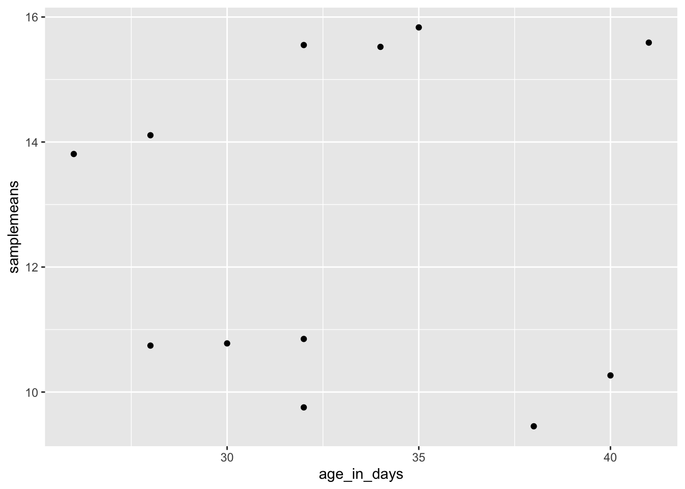
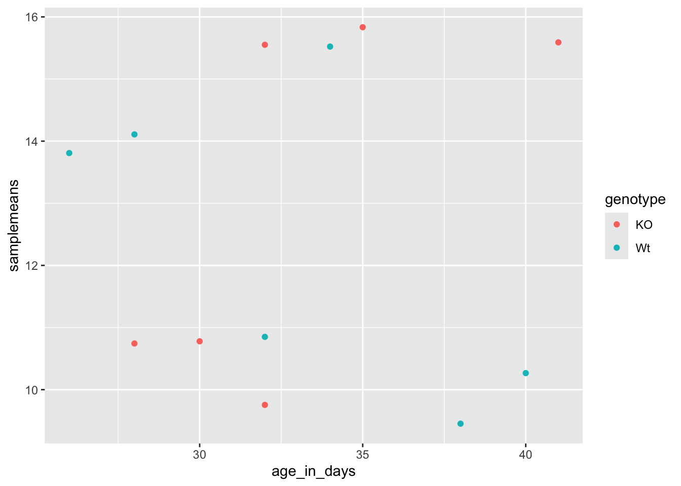
Add color to aesthetics:
Add shape to aesthetics:
ggplot(new_metadata) + geom_point(aes(x = age_in_days, y = samplemeans, color = genotype,
    shape = celltype))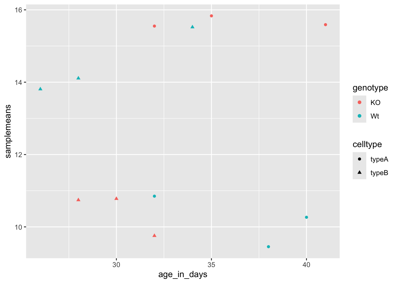
Add point size to geometry:
ggplot(new_metadata) + geom_point(aes(x = age_in_days, y = samplemeans, color = genotype,
    shape = celltype), size = 2.25)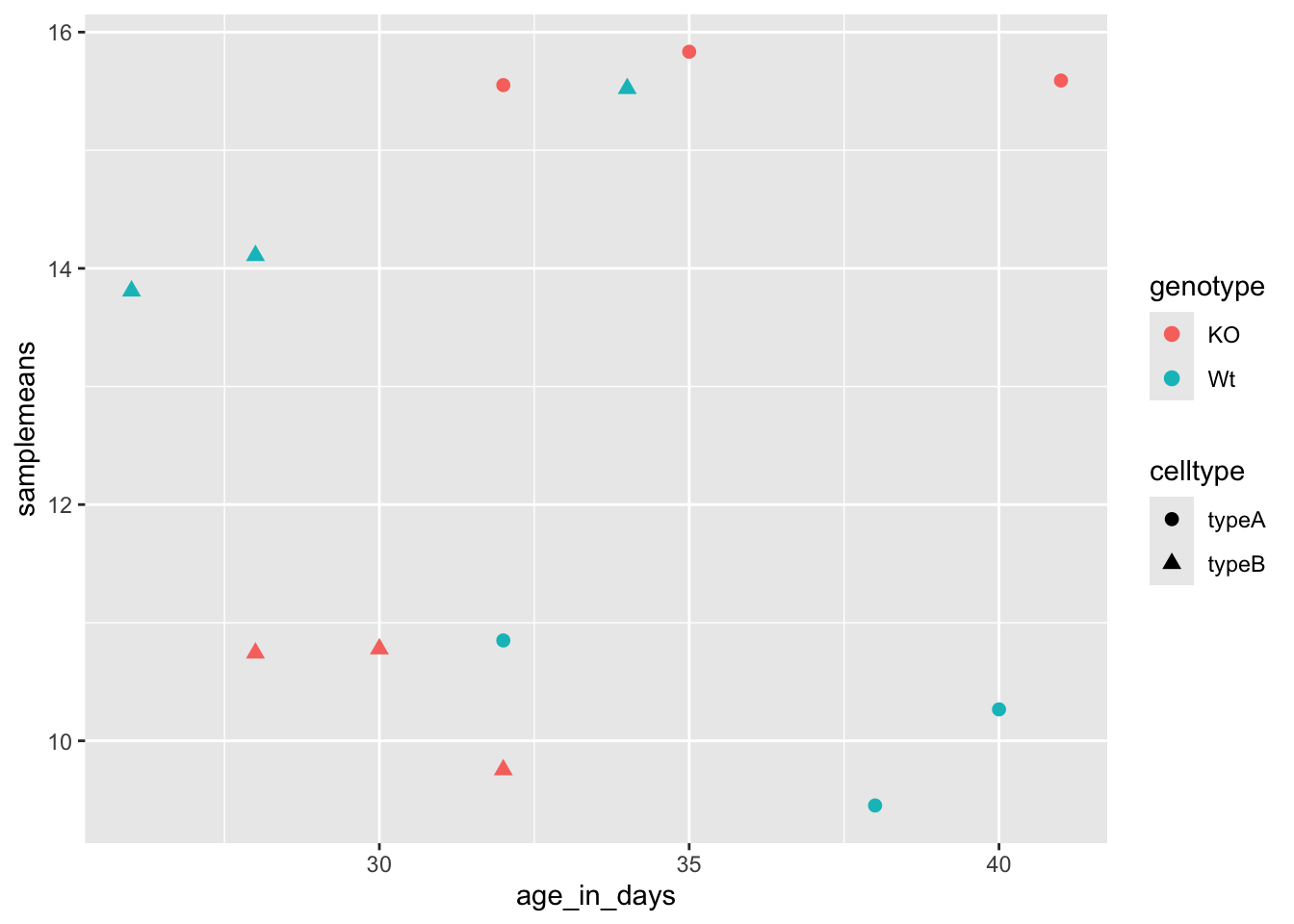
The labels on the x- and y-axis are also quite small and hard to read. To change their size, we need to add an additional theme layer. The ggplot2 theme system handles non-data plot elements such as:
- Axis label aesthetics
- Plot background
- Facet label background
- Legend appearance
5th layer: theme
ggplot(new_metadata) + geom_point(aes(x = age_in_days, y = samplemeans, color = genotype,
    shape = celltype), size = 3) + theme_bw()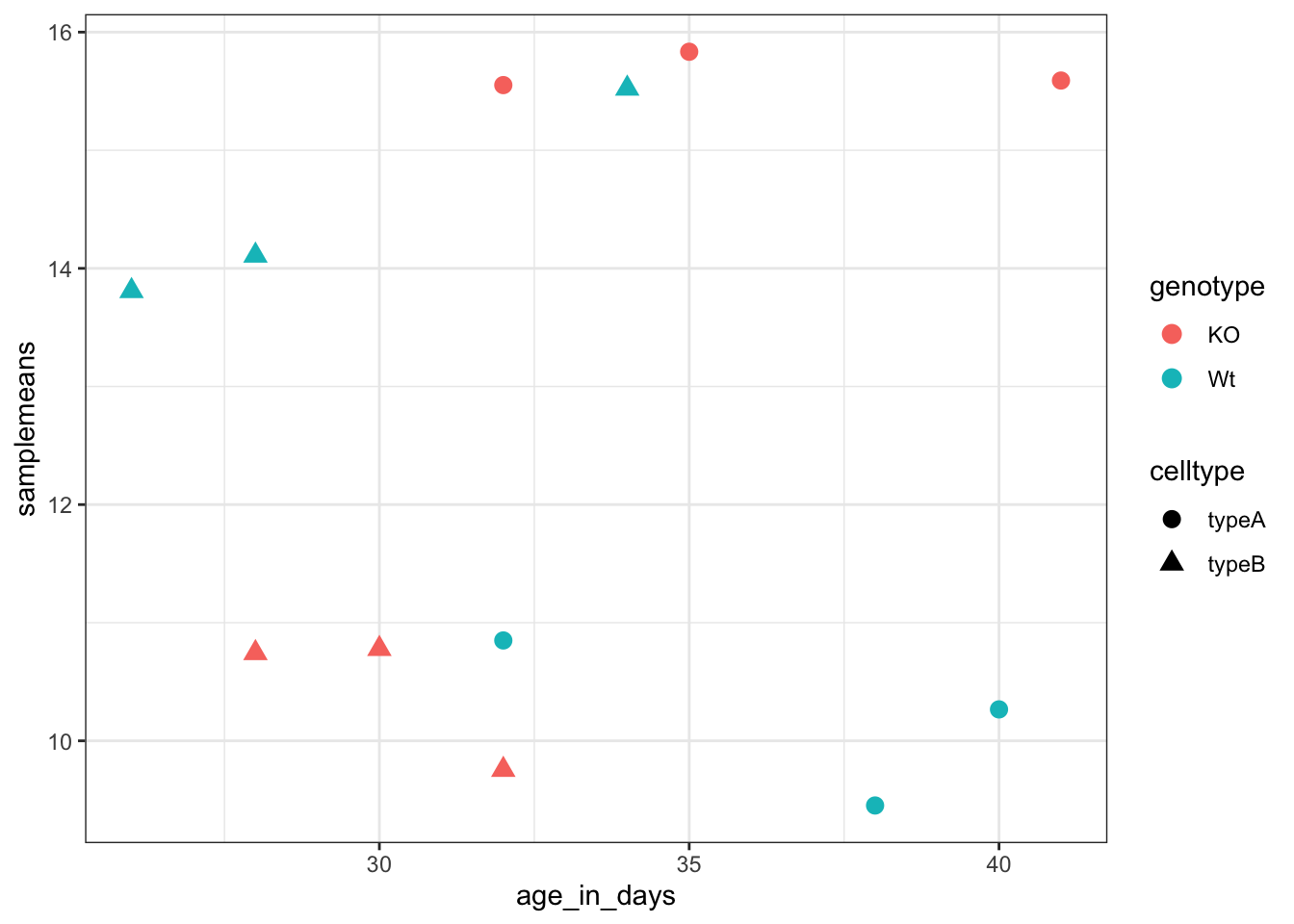
Do the axis labels or the tick labels get any larger by changing themes?
6th layer: axes title size
ggplot(new_metadata) + geom_point(aes(x = age_in_days, y = samplemeans, color = genotype,
shape = celltype), size = 2.25) + theme_bw() + theme(axis.title = element_text(size = rel(1.5))) # increase the size of the axis titles 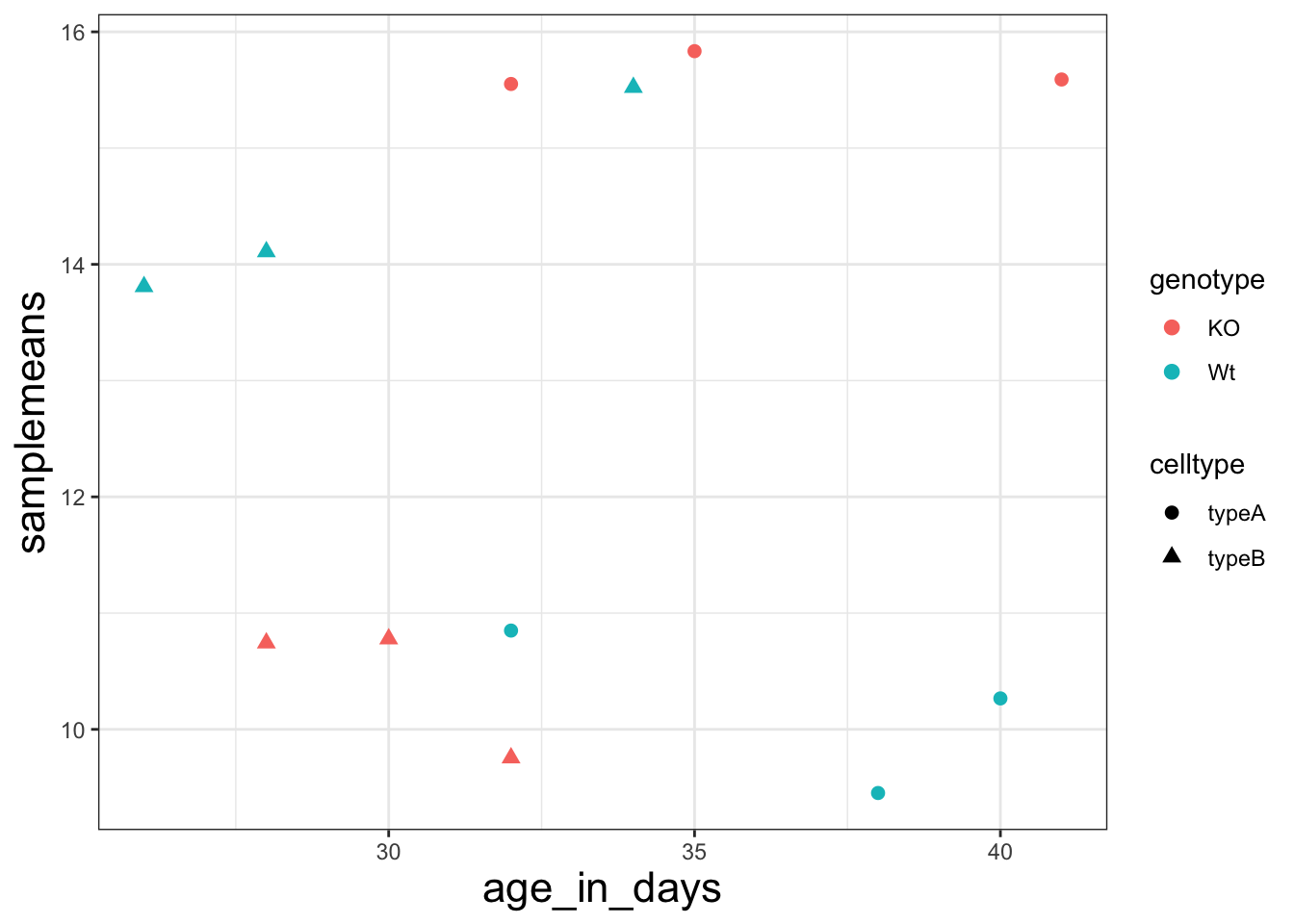
Exercise points +5
The current axis label text defaults to what we gave as input to geom_point (i.e the column headers). We can change this by adding additional layers called xlab() and ylab() for the x- and y-axis, respectively. Add these layers to the current plot such that the x-axis is labeled “Age (days)” and the y-axis is labeled “Mean expression”.
Use the ggtitle layer to add a plot title of your choice.
Add the following new layer to the code chunk: theme(plot.title = element_text(hjust =0.5))
What does it change?
- Ans:
How many theme() layers can be added to a ggplot code chunk, in your estimation?
- Ans:
17.13 13 Boxplot exercise points +16
.md file = 13-boxplot_exercise.md
- Generate a boxplot using the data in the new_metadata dataframe. Create a ggplot2 code chunk with the following instructions:
Use the geom_boxplot() layer to plot the differences in sample means between the Wt and KO genotypes.
Use the fill aesthetic to look at differences in sample means between the celltypes within each genotype.
Add a title to your plot.
Add labels, ‘Genotype’ for the x-axis and ‘Mean expression’ for the y-axis.
Make the following theme() changes:
- Use the theme_bw() function to make the background white.
- Change the size of your axes labels to 1.25x larger than the default.
- Change the size of your plot title to 1.5x larger than default.
- Center the plot title.
- Change genotype order: Factor the
new_metadata$genotypecolumn without creating any extra variables/objects and change the levels toc("Wt", "KO")
- Re-run the boxplot code chunk you created in 1.
- Change default colors
Add a new layer scale_color_manual(values=c(“purple”,“orange”)). Do you observe a change?
- Ans:
Replace scale_color_manual(values=c(“purple”,“orange”)) with scale_fill_manual(values=c(“purple”,“orange”)). Do you observe a change?
- Ans:
In the scatterplot we drew in class, add a new layer scale_color_manual(values=c(“purple”,“orange”)), do you observe a difference?
- Ans:
What do you think is the difference between scale_color_manual() and scale_fill_manual()?
Ans:
Boxplot using “color” instead of “fill”. Use purple and orange for your colors.
- Back in your boxplot code, change the colors in the scale_fill_manual() layer to be your 2 favorite colors.
Are there any colors that you tried that did not work?
- Ans:
- OPTIONAL Exercise
Find the hexadecimal code for your 2 favourite colors (from exercise 3 above) and replace the color names with the hexadecimal codes within the ggplot2 code chunk.
17.14 14 Saving data and plots to file
.md file = 14-exporting_data_and_plots.md
17.14.2 Exporting figures to file:
# opens the graphics device for writing to a file
pdf(file = "figures/scatterplot.pdf")

ggplot(new_metadata) + geom_point(aes(x = age_in_days, y = samplemeans, color = genotype,
    shape = celltype), size = rel(3))

dev.off()  # closes the graphics device
## RStudioGD
## 217.15 15 Finding help
.md file = 15-finding_help.md
17.15.1 Saving variables
In order to find help on line you must provide a reproducible example. Google and R sites such as Stackoverflow are good sources. To provide an example you may want to share an object with someone else, you can save any or all R data structures that you have in your environment to a file.
The function save.image() saves all environmental variables in your current R session to a file called “.RData” in your working directory. This is a command that you should use often when in an R session to save your work.
17.16 16 Tidyverse data wrangling
.md file = 16-tidyverse.md
# If tidyverse is not already installed, uncomment the following line of code
# BiocManager::install('tidyverse')

library(tidyverse)
Tidyverse basics
17.16.1 Pipes: The pipe (%>%) allows the output of a previous command to be used as input to another command instead of using nested functions.
NOTE: Shortcut to write the pipe is shift + command + m on Macos; shift + ctrl + m on Windows
## [1] 9.110434## [1] 9.11## [1] 9.11Exercise points +2
- Create a vector of random numbers using the code below:
Use the pipe (%>%) to perform two steps in a single line:
- Take the mean of random_numbers using the mean() function.
- Round the output to three digits using the round() function.
17.16.2 Tibbles
Experimental data
The dataset: gprofiler_results_Mov10oe.tsv
The gene list represents the functional analysis results of differences between control mice and mice over-expressing a gene involved in RNA splicing. We will focus on gene ontology (GO) terms, which describe the roles of genes and gene products organized into three controlled vocabularies/ontologies (domains):
biological processes (BP)
cellular components (CC)
molecular functions (MF)
that are over-represented in our list of genes.
17.16.3 Analysis goal and workflow
Goal: Visually compare the most significant biological processes (BP) based on the number of associated differentially expressed genes (gene ratios) and significance values and create a plot.
1. Read in the functional analysis results
# Read in the functional analysis results
functional_GO_results <- read.delim(file = "data/gprofiler_results_Mov10oe.tsv")

# Take a look at the results
functional_GO_results[1:3, 1:12]
## query.number significant p.value term.size query.size overlap.size recall
## 1 1 TRUE 0.00434 111 5850 52 0.009
## 2 1 TRUE 0.00330 110 5850 52 0.009
## 3 1 TRUE 0.02970 39 5850 21 0.004
## precision term.id domain subgraph.number
## 1 0.468 GO:0032606 BP 237
## 2 0.473 GO:0032479 BP 237
## 3 0.538 GO:0032480 BP 237
## term.name
## 1 type I interferon production
## 2 regulation of type I interferon production
## 3 negative regulation of type I interferon production## [1] "query.number" "significant" "p.value" "term.size"
## [5] "query.size" "overlap.size" "recall" "precision"
## [9] "term.id" "domain" "subgraph.number" "term.name"
## [13] "relative.depth" "intersection"## [1] "query.number" "significant" "p.value" "term.size"
## [5] "query.size" "overlap.size" "recall" "precision"
## [9] "term.id" "domain" "subgraph.number" "term.name"
## [13] "relative.depth" "intersection"2. Extract only the GO biological processes (BP) of interest
# Return only GO biological processes
bp_oe <- functional_GO_results %>%
dplyr::filter(domain == "BP")
bp_oe[1:3, 1:12]## query.number significant p.value term.size query.size overlap.size recall
## 1 1 TRUE 0.00434 111 5850 52 0.009
## 2 1 TRUE 0.00330 110 5850 52 0.009
## 3 1 TRUE 0.02970 39 5850 21 0.004
## precision term.id domain subgraph.number
## 1 0.468 GO:0032606 BP 237
## 2 0.473 GO:0032479 BP 237
## 3 0.538 GO:0032480 BP 237
## term.name
## 1 type I interferon production
## 2 regulation of type I interferon production
## 3 negative regulation of type I interferon productionNote: the dplyr::filter is necessary because the stats library gets loaded with ggplot2, rmarkdown and bookdown and stats also has a filter function
Exercise points +1
We would like to perform an additional round of filtering to only keep the most specific GO terms.
- For bp_oe, use the filter() function to only keep those rows where the relative.depth is greater than 4.
- Save output to overwrite our bp_oe variable.
17.16.4 Select
- Select only the colnames needed for visualization
##  [1] "query.number"    "significant"     "p.value"         "term.size"
##  [5] "query.size"      "overlap.size"    "recall"          "precision"
##  [9] "term.id"         "domain"          "subgraph.number" "term.name"
## [13] "relative.depth" "intersection"bp_oe <- bp_oe %>%
select(term.id, term.name, p.value, query.size, term.size, overlap.size, intersection)
head(bp_oe[, 1:6])## term.id term.name p.value query.size
## 1 GO:0090672 telomerase RNA localization 2.41e-02 5850
## 2 GO:0090670 RNA localization to Cajal body 2.41e-02 5850
## 3 GO:0090671 telomerase RNA localization to Cajal body 2.41e-02 5850
## 4 GO:0071702 organic substance transport 7.90e-11 5850
## 5 GO:0015931 nucleobase-containing compound transport 4.43e-05 5850
## 6 GO:0050657 nucleic acid transport 3.67e-06 5850
## term.size overlap.size
## 1 16 11
## 2 16 11
## 3 16 11
## 4 2629 973
## 5 200 93
## 6 166 83## [1] 668 717.16.6 Rename
Let’s rename the term.id and term.name columns.
# Provide better names for columns
bp_oe <- bp_oe %>%
    dplyr::rename(GO_id = term.id, GO_term = term.name)
Exercise points +1
Rename the intersection column to genes to reflect the fact that these are the DE genes associated with the GO process.
17.16.7 Mutate
Create additional metrics for plotting (e.g. gene ratios)
# Create gene ratio column based on other columns in dataset
bp_oe <- bp_oe %>%
    mutate(gene_ratio = overlap.size/query.size)
Exercise points +1
Create a column in bp_oe called term_percent to determine the percent of DE genes associated with the GO term relative to the total number of genes associated with the GO term (overlap.size / term.size)
Gives you a sense of how many of the genes in the GO term are differentially expressed.
Exercise points +4
Use ggplot to plot the first 30 significant GO terms vs gene_ratio. Color the points by p.value as shown in the figure in below:
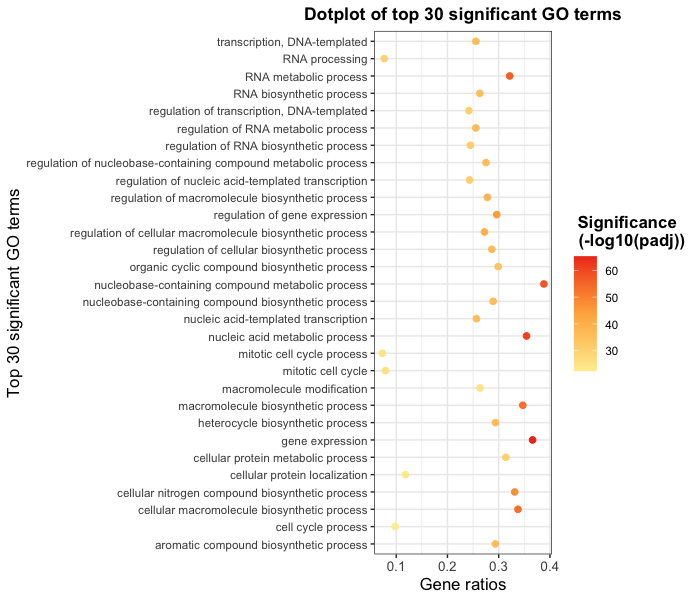
Change the p.value gradient colors to red-orange-yellow
# to help linearize the p.values for the colors; not essential for answer
sub$`-log10(p.value)` = -log10(sub$p.value)
# Your code here
See ggplot for more detail.