Chapter 2 Introduction to R and RStudio
2.1 What is R?
R is a programming language and is a great option for analyzing and visualizing data. R is open source and has an active development community that’s constantly releasing new packages, making R code even easier to use.

2.3 Open a project directory in RStudio
Start Rstudio, and go to the
Filemenu, selectOpen Project, and navigate to your 2024_IntroR_and_RStudio folder and double click on2024_IntroR_and_RStudio.Rproj.When RStudio opens, you will see four panels in the window.
Open the file
17-introR_codebook.Rmdin the lessons directory under the File menu (lower right panel). It will open in the script window in the upper left. This file contains all the R code that we will be running in the lessons.
2.4 RStudio Interface
The RStudio interface has four main panels:
Console: (lower left panel) where you can type commands and see output.
Script editor: (upper left panel) where you can type out commands and save to file. You can also submit the commands to run in the console.
Environment/History/Git: (upper right panel)
Environment: lists the active objects in your R session
History: keeps track of all commands run in console.
Git keeps track of any changes in your git repository. It is important that you don’t change any of the original files in your working directory. In fact, it’s best if you save
17-introR_codebook.Rmdwhich contains all the code we will be running under another name, e.g.17-codebook_yourname.Rmd, with your name at the end. You can save this either in the lessons directory or in the scripts directory, this is the document you will be handing in as your homework for this module. This way you can always go back to the original file if you need to. If you want to take notes, you can do so in the17-codebook_yourname.Rmdfile.
- Files/Plots/Packages/Help (lower right panel)
File: lists all the files in your project directory (current directory)
Plots: shows the output of graphs you generate – set the output of your Rmd file to “Preview in Viewer Pane”; cogwheel next to Knitr button at the top of your window.
Packages: lists the loaded libraries
Help: interface for R help menu for functions and packages
2.5 Interacting with R
There are two main ways of interacting with R in RStudio: using the console or by using script editor (plain text files that contain your code).
2.5.1 Console window
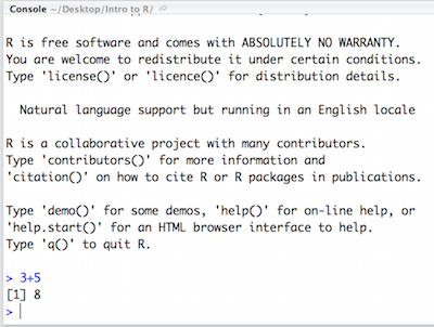
The console window (in RStudio, the bottom left panel) is the place where R will show the results of a command. You can type commands directly into the console, but they will be forgotten when you close the session.
Let’s test it out; in your console type:

2.5.2 Script editor
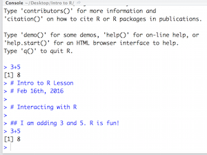
You can use the comments character # to add additional descriptions.t It’s best practice to comment liberally to describe the commands you are running using #. To run the code, you click on the little green arrow on the side of the code chunk. Let’s run the second chunk.
You will see the command run in the console and output the result.
You can also run the code by highlighting it and pressing the Ctrl and Return/Enter keys at the same time as a shortcut.

2.6 The R syntax
Now that we know how to talk with R via the script editor or the console, we want to use R for something more than adding numbers. To do this, we need to know more about the R syntax.
The main parts of R (syntax) include:
the comments
#and how they are used to document function and its contentvariables and functions
the assignment operator
<-the
=for arguments in functions
We will go through each of these in more detail, starting with the assignment operator.
2.7 Assignment operator
To do useful and interesting things in R, we need to assign values to
variables using the assignment operator, <-. For example, we can use the assignment operator to assign the value of 3 to x by executing:
The assignment operator (<-) assigns values on the right to variables on the left.
In Windows, typing Alt + - (push Alt at the same time as the - key, on Mac type option + -) will write <- in a single keystroke.
2.8 Variables
In the example above, we created a variable called xand assigned it a value of 3.
Let’s create another variable called y and give it a value of 5.
You can view information on the variable by looking in your Environment window in the upper right-hand corner of the RStudio interface.

Now we can reference these variables by name to perform mathematical operations on the values contained within. What do you get in the console for the following operation:
Try assigning the results of this operation to another variable called number.
Exercises
Try changing the value of the variable
xto 5. What happens tonumber?Now try changing the value of variable
yto contain the value 10. What do you need to do, to update the variablenumber?
2.8.1 Tips on variable names
Variables can be given almost any name, such as x, current_temperature, or
subject_id. However, there are some rules / suggestions you should keep in mind:
Avoid names starting with a number (
2xis not valid butx2is)Avoid dots (
.) within a variable name; dots have a special meaning in R (for methods) so it’s best to avoid them.Keep in mind that R is case sensitive (e.g.,
genome_lengthis different fromGenome_length)Be consistent with the styling of your code (where you put spaces, how you name variable, etc.). In R, two popular style guides:
2.9 Interacting with data in R
R is commonly used for handling big data, and so it only makes sense that we learn about R in the context of some kind of relevant data.
2.9.1 Data directory
You can access the files we need for this workshop in your data directory. We will discuss these files a bit later in the lesson.
2.9.2 The mouse dataset
In this example dataset we have collected whole brain samples from 12 mice and want to evaluate expression differences between them. The expression data represents normalized count data (normalized_counts.txt) obtained from RNA-sequencing of the 12 brain samples. This data is stored in a comma separated values (CSV) file as a 2-dimensional matrix, with each row corresponding to a gene and each column corresponding to a sample.

2.9.3 The metadata
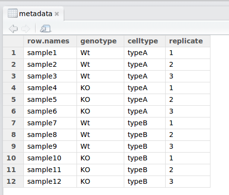
We have another file in which we identify information about the data or metadata (mouse_exp_design.csv). Our metadata is also stored in a CSV file. In this file, each row corresponds to a sample and each column contains some information about each sample.
The first column contains the row names, and note that these are identical to the column names in our expression data file above (albeit, in a slightly different order). The next few columns contain information about our samples that allow us to categorize them. For example, the second column contains genotype information for each sample. Each sample is classified in one of two categories: Wt (wild type) or KO (knockout). What types of categories do you observe in the remaining columns?

These lessons have been developed by members of the teaching team at the Harvard Chan Bioinformatics Core (HBC). These are open access materials distributed under the terms of the Creative Commons Attribution license (CC BY 4.0), which permits unrestricted use, distribution, and reproduction in any medium, provided the original author and source are credited.
