tlcdata <- readRDS("data/tlc.RDS")
head(tlcdata)
id treatment week lead
1 1 placebo 0 30.8
101 1 placebo 1 26.9
201 1 placebo 4 25.8
301 1 placebo 6 23.8
2 2 succimer 0 26.5
102 2 succimer 1 14.8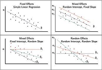
Reading
Basic Concepts
Mixed models for data that are not independent, e.g. repeated measures or clustered data.
Correlated data: multiple observations on individuals, i.e., “units”, “groups”, “clusters”.
Correlated data allows us (at minimum) to gain information about the variability of measurements on individuals.
The cost of correlated data is that each additional correlated individual contributes less information than the previous one, and much less than a single person in a new cluster.
Longitudinal data: Measurements on the same individual are made repeatedly over time- a type of correlated data.
Multilevel data: Individuals are nested within groups.
Random intercept model: motivation and interpretation
Shrinkage estimation and BLUPs of random effects.
Random slope model
Hierarchical formulation of random effect model.
tlcdata <- readRDS("data/tlc.RDS")
head(tlcdata) id treatment week lead
1 1 placebo 0 30.8
101 1 placebo 1 26.9
201 1 placebo 4 25.8
301 1 placebo 6 23.8
2 2 succimer 0 26.5
102 2 succimer 1 14.8library(ggplot2)
library(dplyr)
library(gridExtra)
placebo <- tlcdata %>%
filter(treatment == "placebo") %>%
ggplot() +
geom_line(aes(x = week, y = lead, col = id)) +
labs(x = "Week", y="Lead", title = "Placebo") +
theme(legend.position = "none")
succimer <- tlcdata %>%
filter(treatment == "succimer") %>%
ggplot() +
geom_line(aes(x = week, y = lead, col = id, linetype = treatment)) +
labs(x = "Week", y="Lead",title = "Succimer") +
theme(legend.position = "none")
gridExtra::grid.arrange(placebo, succimer)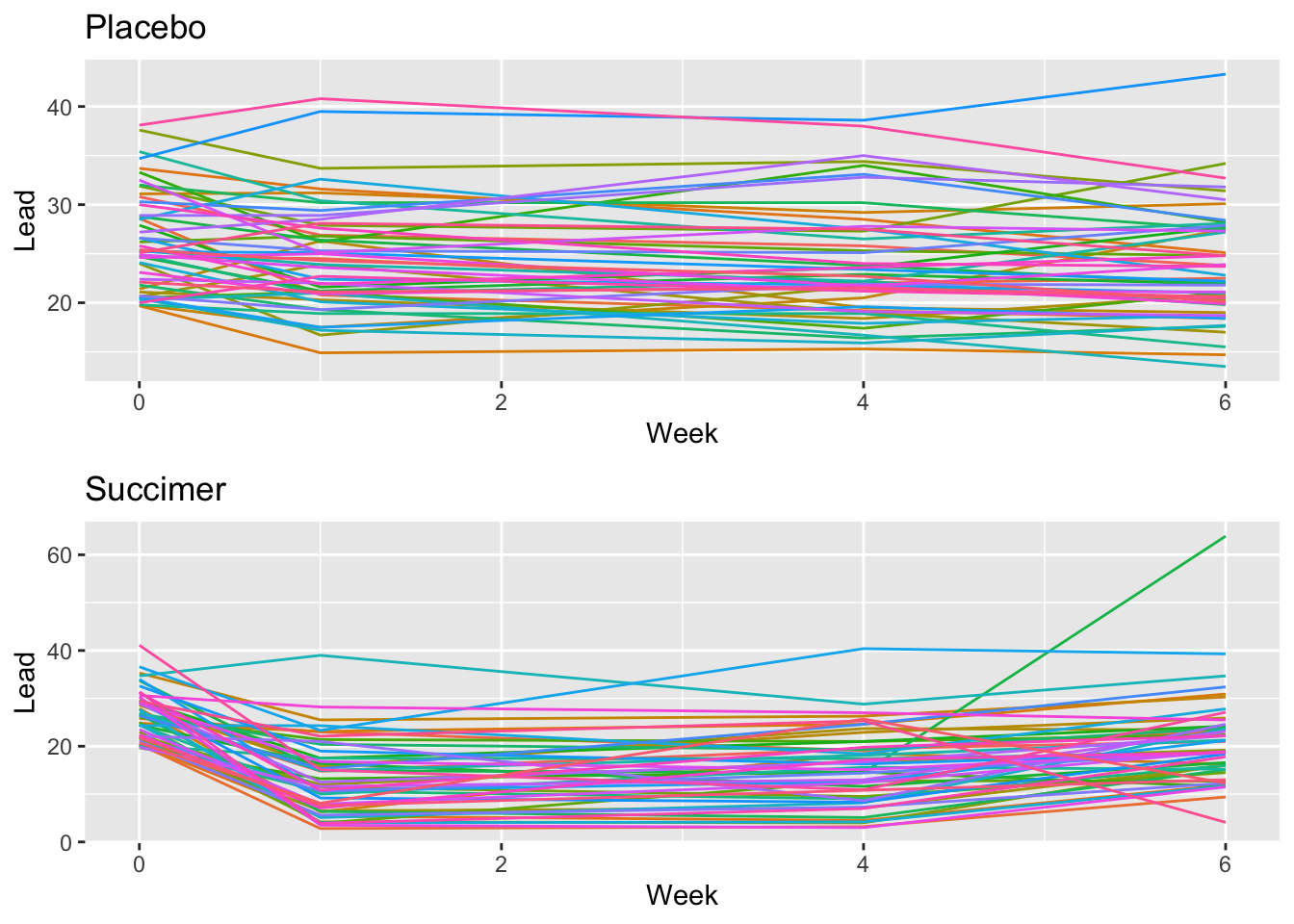
![]()
fit.lm = lm(lead ~ week, data = tlcdata)
summary(fit.lm)
Call:
lm(formula = lead ~ week, data = tlcdata)

Residuals:
    Min      1Q  Median      3Q     Max
-19.775  -3.749   0.328   4.454  43.330

Coefficients:
            Estimate Std. Error t value Pr(>|t|)
(Intercept)  22.9760     0.6079  37.793   <2e-16 ***
week         -0.4010     0.1670  -2.401   0.0168 *
---
Signif. codes:  0 '***' 0.001 '**' 0.01 '*' 0.05 '.' 0.1 ' ' 1

Residual standard error: 7.966 on 398 degrees of freedom
Multiple R-squared:  0.01428,   Adjusted R-squared:  0.0118
F-statistic: 5.765 on 1 and 398 DF, p-value: 0.01681![]()
If observations were uncorrelated, i.e., if we had measured different subjects at 0, 1, 4, and 6 weeks post-exposure, then we could fit the standard linear model:
There is an indicator for each time point, where
BUT the data are correlated. How do we handle this?
We extend the linear model to allow correlation (covariance).
A Better Approach: Linear Mixed Models
LMMs are extensions of regression in which intercepts and/or slopes are allowed to vary across individuals.
Mixed models were developed to deal with correlated data.
They allow for the inclusion of both fixed and random effects.
Fixed effect: a global or constant parameter that does not vary.
Random effect: Parameters that are random variables and are assigned a distributional assumption, e.g.,
Taking our motivating example, we can assign a separate intercept for each child:
Limitations:
Estimating lots of parameters: subject-specific coefficients do not leverage overall population information and have less precision because of smaller sample size.
Cannot forecast the grow curve of a new child.
We treat the “group” or “nested” unit as a factor/dummy variable. Therefore, we DO NOT include the intercept (see Module 1). Including the “cluster” as a factor allows for individual intercepts across children. Use the
fit.strat = lm(lead ~week + factor(id)-1, data =tlcdata) #do not include the intercept!!
summary(fit.strat$coefficients[1])
Min. 1st Qu. Median Mean 3rd Qu. Max.
-0.401 -0.401 -0.401 -0.401 -0.401 -0.401 summary(fit.strat$coefficients[2]) Min. 1st Qu. Median Mean 3rd Qu. Max.
27.93 27.93 27.93 27.93 27.93 27.93 Data are balanced (same number of observations for each child).
The slope of week is the same in the model with a single intercept and the model with child-specific intercepts.
Controlling for group-specific intercepts gives a smaller standard error for the slope of week because week is the same for all children.
Note that oftentimes, the standard error will be larger if there is sparse or unbalanced data.
What is the interpretation of
![]()
Consider the random intercept model with a vector of predictors
What makes this a mixed model?
The following two models are equivalent:
Model 1:
Model 2: The hierarchical model framework
Model 2 is an example of a hierarchical model in which there are hierarchical structures placed on random effects. Here the random coeffcient
Assumptions:
What is the overall (average) trend?
What is total variability around the overall trend?
What is the conditional (group-specific) trend?
What is the conditional (within-group) residual variance?
![]()
library(lmerTest)Loading required package: lme4Loading required package: Matrix
Attaching package: 'lmerTest'The following object is masked from 'package:lme4':
lmerThe following object is masked from 'package:stats':
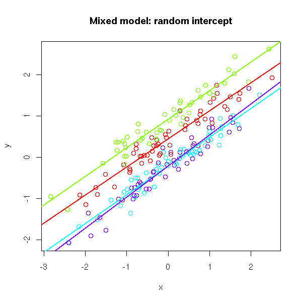
stepfit.randomeffects = lmer(lead ~ week + (1|id), data = tlcdata)
summary(fit.randomeffects)Linear mixed model fit by REML. t-tests use Satterthwaite's method [
lmerModLmerTest]
Formula: lead ~ week + (1 | id)
Data: tlcdata
REML criterion at convergence: 2695.1
Scaled residuals:
Min 1Q Median 3Q Max
-2.6337 -0.3461 0.0601 0.4131 6.1167
Random effects:
Groups Name Variance Std.Dev.
id (Intercept) 29.63 5.444
Residual 33.98 5.829
Number of obs: 400, groups: id, 100
Fixed effects:
Estimate Std. Error df t value Pr(>|t|)
(Intercept) 22.9760 0.7030 161.6442 32.683 < 2e-16 ***
week -0.4010 0.1222 299.0000 -3.281 0.00116 **
---
Signif. codes: 0 '***' 0.001 '**' 0.01 '*' 0.05 '.' 0.1 ' ' 1
Correlation of Fixed Effects:
(Intr)
week -0.478#Extracting the random effects theta_i's
random.eff = ranef(fit.randomeffects)$id
hist(random.eff$`(Intercept)`)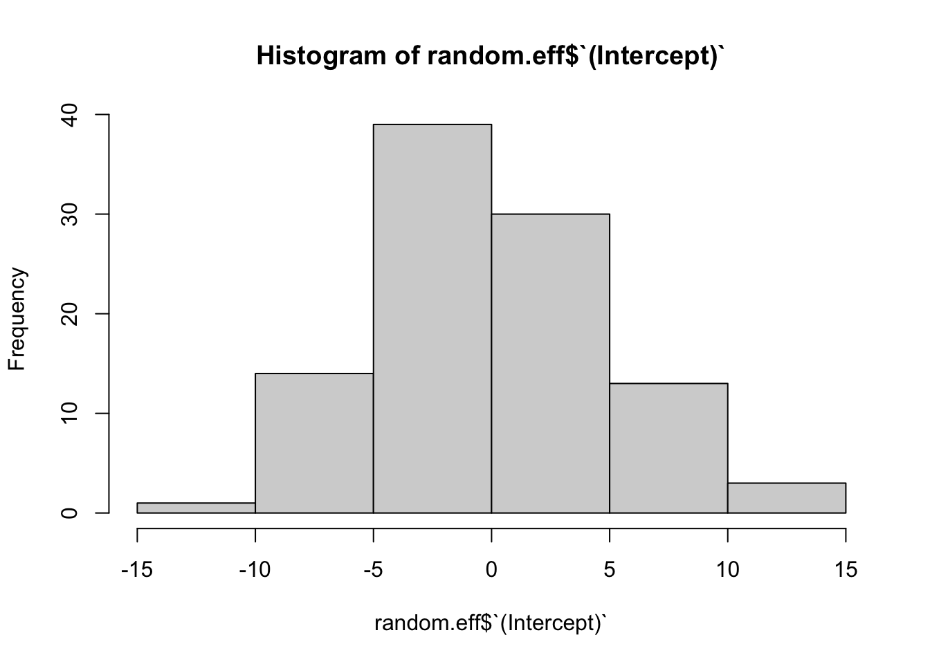
Let’s fit an alternative model to the data including a treatment effect:
library(lmerTest)
fit.randomeffects = lmer(lead ~ week + treatment +  (1|id), data = tlcdata)
summary(fit.randomeffects)
Linear mixed model fit by REML. t-tests use Satterthwaite's method [
lmerModLmerTest]
Formula: lead ~ week + treatment + (1 | id)
Data: tlcdata
REML criterion at convergence: 2670.2
Scaled residuals:
Min 1Q Median 3Q Max
-2.4885 -0.3686 -0.0176 0.4514 6.3428
Random effects:
Groups Name Variance Std.Dev.
id (Intercept) 22.09 4.700
Residual 33.98 5.829
Number of obs: 400, groups: id, 100
Fixed effects:
Estimate Std. Error df t value Pr(>|t|)
(Intercept) 25.7648 0.8512 136.0165 30.269 < 2e-16 ***
week -0.4010 0.1222 299.0000 -3.281 0.00116 **
treatmentsuccimer -5.5775 1.1060 98.0000 -5.043 2.1e-06 ***
---
Signif. codes: 0 '***' 0.001 '**' 0.01 '*' 0.05 '.' 0.1 ' ' 1
Correlation of Fixed Effects:
(Intr) week
week -0.395
trtmntsccmr -0.650 0.000What are the overall findings from this model? And how does this model differ from the previous model?
![]()
![]()
Consider the mixed model with random intercepts for
where
| What is the model? |
|
| Model Assumptions |
|
| Interpretation |
|
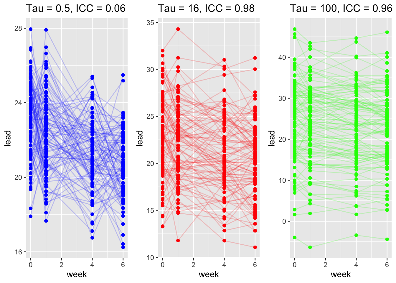
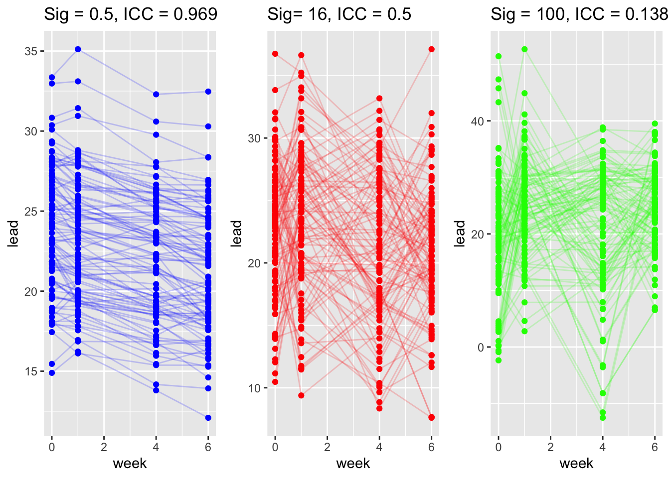
Note that the within-group covariance is:
So the correlation between observations within within the same group is
![]()
Now consider the matrix formulation
Given the values of
![]()
Note that:
Taking the first derivative, setting to 0, and solve! (On your own time).
Since
We can also express
Less shrinkage is expected for
For unknown variance parameters
Note that
The MLE estimate of the variances is biased! (Similar to the estimate in simple linear regression).
An alternative is the restricted maximum likelihood (REML):
vs.
$_{0i} = _0 + $ participant specific intercept or child specific average.
What do we do for
![]()
Let’s fit the model using the tlc data:
placebo_data = tlcdata %>% filter(treatment == "placebo")
fit_random <- lmer(lead ~ week + (week|id), data = placebo_data)
summary(fit_random)
Linear mixed model fit by REML. t-tests use Satterthwaite's method [
lmerModLmerTest]
Formula: lead ~ week + (week | id)
Data: placebo_data
REML criterion at convergence: 1053.3
Scaled residuals:
Min 1Q Median 3Q Max
-2.20808 -0.49837 -0.02268 0.47100 2.30541
Random effects:
Groups Name Variance Std.Dev. Corr
id (Intercept) 23.3113 4.8282
week 0.1581 0.3976 0.02
Residual 4.5016 2.1217
Number of obs: 200, groups: id, 50
Fixed effects:
Estimate Std. Error df t value Pr(>|t|)
(Intercept) 25.68536 0.72018 49.01076 35.665 < 2e-16 ***
week -0.37213 0.08437 49.00066 -4.411 5.64e-05 ***
---
Signif. codes: 0 '***' 0.001 '**' 0.01 '*' 0.05 '.' 0.1 ' ' 1
Correlation of Fixed Effects:
(Intr)
week -0.164AIC: Akaike’s Information Criterion.
AIC is often used in model selection. It is a popular approach to choosing which variables should be in the model.
The MLE estimate of the variances is biased! (Similar to the estimate in simple linear regression).
The general rule of thumb is a differenc of 2+ is substantially better. A lower AIC is better.
The AIC uses the maximum likelihood so use
load("/Users/emilypeterson/Library/CloudStorage/OneDrive-EmoryUniversity/BIOS 526/BIOS526_Book/data/Nepal200.RData")