Module 5 Part 2: Penalized and Smoothing Splines

Reading

• Chapter 5- Elements of Statistical Learning (Hastie)

• Chapter 5- Introduction to Statistical Learning (James et al. )

Basic Concepts

• Constraints and penalized regression
• Smoothing matrix and smoothing parameter
• Generalized cross-validation to choose roughness penalty
• Mixed models to choose roughness penalty

Parametric Splines

Motivating Example: Daily Temperature and Deaths

• all deaths: daily non-accidental deaths in the 5 county New York City 2001-2005.

• temp: daily temperature (Fahrenheit)

Regression Problem

• Let \(y_i\) be the number of non-accidental deaths on day \(i\) and \(x_i\) be the same-day temperature.

• We consider the nonparametric regression problem:

\[ y_i = g(x_i) + \epsilon_i, \quad \epsilon_i \overset{iid}{\sim} (0, \sigma^2) \]

• We can approximate \(g(x_i)\) using a generalized additive model: \[ y_i = \beta_0 + \sum_{m=1}^M \beta_m b_m(x_i) + \epsilon_i, \quad \epsilon_i \overset{iid}{\sim} (0, \sigma^2) \]

e.g., linear spline with 9 equidistant interior knots, \(\kappa_1, \kappa_2, ..., \kappa_9\) within the observed range of daily temps, a piecewise linear spline model:

\[ \begin{align*} g(x_i) &= \beta_0 + \beta_1 x_i + \beta_2 (x_i - \kappa_1 )_{+} + ... + \beta_10 (x_i - \kappa_9)_{+}\\ (x_i - \kappa_m)_{+} &= \begin{cases} (x_i-\kappa_m),& \text{ if } x_i \geq \kappa_m\\ 0 & \text{otherwise} \end{cases} \end{align*} \]

Lets fit this to the data:

library(splines)
library(dplyr)

Attaching package: 'dplyr'

The following objects are masked from 'package:stats':

    filter, lag

The following objects are masked from 'package:base':

    intersect, setdiff, setequal, union

library(tidyr)

# Define 9 evenly spaced knots
knots <- seq(min(health$Temp), max(health$Temp), length.out = 9)

# Create a linear spline basis using bs() function
spline_basis <- bs(health$Temp, knots = knots[-c(1, length(knots))], degree = 1) # Exclude boundary knots

# Fit a linear model with the spline basis
fit <- lm(alldeaths ~ spline_basis, data = health)


# Plot the results
plot(health$Temp, health$alldeaths, main = "Linear Spline with 9 Knots", col = "grey", pch = 16, xlab = "Temp", ylab = "Death Count")
lines(health$Temp, predict(fit), col = "blue", lwd = 2)
abline(v = knots, col = "red", lty = 2) # Show knot locations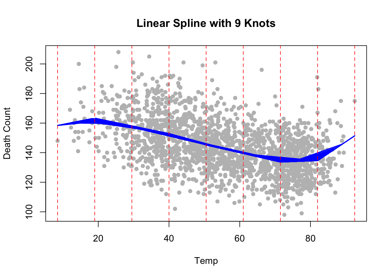

Automatic Knot Selection

What if we don’t know the number and locations of the knots?

Splines can overfit the data when number of knot increases. We want to avoid overfitting

Approach

• Start with a lot of knots. This ensures we will not miss important fine-scale behavior.
• Assume most of the knots are not useful and shrink their coefficients towards zero.
• Determine how much to shrink based on some criteria (e.g. CV, GCV, AIC).

Benefits

• Knot placement is not important if the number is dense enough.
• Shrinking most coefficients to zero will stabilize model estimation similar to performing variable selection.

Penalized Spline

Consider the basis expansion :

\[ g(x_i) = \beta_0 + \beta_1 x_i + \sum_{m=1}^M \beta_{m_+1} b)m(x_i) \] - Constrain the magnitude of the coefficients \(\beta_j\). - Consider the ridge regression penalty:

\[ \beta_2^2 + \beta_3^2 + ... + \beta_{M+1}^2 \leq C \] equivalently \(||\beta^*||_2^2 \leq C\) where \(||\beta^*||_2\) is the L2-norm and where \(\beta^* = [\beta_2, ..., \beta_{M+1}]'\) and \(C\) is a positive constant.

Important

L2 Definition: The L2 norm, also called the Euclidean norm, is a measure of the magnitude (or length) of a vector in Euclidean space. It is defined as:

\[ \|\mathbf{v}\|_2 = \sqrt{v_1^2 + v_2^2 + \dots + v_n^2} = \sqrt{\sum_{i=1}^n v_i^2} \]

where \(\mathbf{v} = [v_1, v_2, \dots, v_n]\) is a vector in \(\mathbb{R}^n\).

The L2 norm is the square root of the sum of the squared elements of the vector.

Properties:

1. Non-Negativity

\[ \|\mathbf{v}\|_2 \geq 0 \]

• \(\|\mathbf{v}\|_2 = 0\) if and only if \(\mathbf{v} = 0\).

2. Scalability: If \(c\) is a scalar:

\[ \|c \mathbf{v}\|_2 = |c| \cdot \|\mathbf{v}\|_2 \]

3. Triangle Inequality: For two vectors $ $ and \(\mathbf{v}\):

\[ \|\mathbf{u} + \mathbf{v}\|_2 \leq \|\mathbf{u}\|_2 + \|\mathbf{v}\|_2 \]

4. Geometric Interpretation: The L2 norm corresponds to the Euclidean distance from the origin to the point \(\mathbf{v}\) in \(n\)-dimensional space. For a 2D vector \(\mathbf{v} = [x, y]\), the L2 norm is:

\[ \|\mathbf{v}\|_2 = \sqrt{x^2 + y^2} \]

This is the standard distance formula in 2D geometry.

Penalties

• Ridge regression \(= \text{L2- penalty} = ||\beta^*||_2^2\).

  • Ridge shrinks coefficients of vectors in B-spline basis, but does not induce sparsity.
  • Ridge is easy to solve- closed form solution!

• Lasso = absolute value = \(\text{L1-penalty } = ||\beta^*||_1 = \sum_{j=2}^{M+1} |\beta_j|\).

  • Lasso tends to make some coefficients exactly zero.
  • Trickier to solve. More on this later.

• A small \(C\) will shrink more coefficients, as well as shrink them closer to zero.

• Our goal: Convert the two problems: (1) number of knots, and (2) their location- into a single parameter that we can choose with GCV.

Matrix of \(g()\)

• For simplicity, consider a linear spline. Then evaluate the basis functions at each \(x_i, i=1,...,n\) resulting the following matrix.

\[ X = \begin{bmatrix} 1 & x_1 & (x_1 - \kappa_1)_+ & \cdots & (x_1 - \kappa_{M+1})_+ \\ 1 & x_2 & (x_2 - \kappa_1)_+ & \cdots & (x_2 - \kappa_{M+1})_+ \\ \vdots & \vdots & \vdots & \ddots & \vdots \\ 1 & x_n & (x_n - \kappa_1)_+ & \cdots & (x_n - \kappa_{M+1})_+ \end{bmatrix} \]

where:

• \(\kappa_1, \dots, \kappa_{M+1}\) are the knot points,
• \((x - \kappa)_+\) denotes the positive part function:

\[ (x - \kappa)_+ = \begin{cases} x - \kappa, & \text{if } x > \kappa, \\ 0, & \text{if } x \leq \kappa. \end{cases} \]

Writing \(g(x_i)\) in Matrix Form: The function \(g(x_i),i = 1, \dots, n\), can be written in matrix form as:

\[ \begin{align*} g(x)& = X \beta,\\ g(x_i) & = \beta_0 + \beta_1 x_i + \sum_{m=1}^M B_{m+1} (x_i - \kappa_m)_+ \end{align*} \]

where \(\beta\) is the vector of coefficients.

Residuals are given by:

\[ Y - G = Y - X \beta, \]

where \(Y\) is the response vector, \(G\) represents the fitted values, and \(X \beta\) is the estimated spline fit.

Constrained Formulation

Important

We define the objective function as:

\[ \text{argmin}_{\beta} \quad (Y - X\beta)'(Y - X\beta) \quad \text{subject to} \quad \beta'B\beta \leq C. \]

The term \((Y - X\beta)'(Y - X\beta)\) represents the residual sum of squares (RSS) or the squared error term. Measure of model fit.

• Smaller values indicate a better fit.
• Want to minimize RSS, i.e., find \(\beta\) that makes the model predictions \(X\beta\) close to observed \(y\).

Constraint :

The constraint \(\beta'B\beta \leq C\) imposes a penalty on the coefficients \(\beta\):

• \(\beta'B\beta\) is a quadratic form, where \(B=\) a diagonal matrix with 0s and 1s.
• \(B\) selects which coefficients are penalized:
  • 1 in \(B\) means that the corresponding coefficient in this \(\beta\) is penalized.
  • 0 in \(B\) means the corresponding coefficient is not penalized.
• \(C\) is a threshold that limits the total magnitude of the penalized coefficients.

Penalty Formulation

Important

This problem can be equivalently formulated without constraint \(C\) as

\[ \text{argmin}_{\beta} \quad (Y - X\beta)'(Y - X\beta) + \overset{\text{penalty function}}{\lambda \beta'B\beta} \]

There is a one-to-one mapping between \(\lambda\) and the constraint \(C\), i.e., for each \(\lambda\) you can find a corresponding \(C\).

• The smoothing parameter, \(\lambda\), controls the trade-off between:

  • Minimizing the residual sum of squares (fit to the data).
  • Penalizing complexity of the model (regularization term \(\beta'B\beta\)).

• A larger value of \(\lambda\) increases the penalty, resulting in a smoother (less complex) model.

• A smaller value of $$ allows more flexibility, potentially fitting the data more closely but risking overfitting.

• Why This Matters

  • Constraint-based and penalty-based—are equivalent in theory but have different practical uses:
  • Constraint-based Formulation: Useful for explicitly enforcing a limit on model complexity (e.g., in constrained optimization problems).
  • Penalty-based Formulation: Easier to solve using standard optimization techniques and more common in regularization methods like Ridge Regression or Smoothing Splines.

Closed-Form Solution

1. The optimization problem is defined as:

\[ \text{argmin}_{\beta} \quad (Y - X\beta)'(Y - X\beta) + \lambda \beta'B\beta. \]

2. Differentiating with Respect to \(\beta\):

To find the closed-form solution, differentiate the objective function with respect to \(\beta\) and set it to zero:

\[ -2X'(Y - X\beta) + 2\lambda B\beta = 0. \]

3. Simplify:

\[ -X'Y + X'X\beta + \lambda B\beta = 0. \]

4. Rearranging terms:

\[ (X'X + \lambda B)\beta = X'Y. \]

5. Final Solution: Solving for \(\beta\) gives least squares solution:

\[ \hat{\beta} = (X'X + \lambda B)^{-1}X'Y. \]

for some positive number \(\lambda\). Note:

• When \(\lambda=0\) \(\hat{\beta}\) becomes OLS estimate. So no penalization and \(C=\infty)\).
• When \(\lambda\rightarrow \infty\), \((X'X + \lambda b)^{-1}\)a becomes small, so \(\hat{\beta}_j \rightarrow 0\).
• Note here \(\hat{\beta}_0\) and \(\hat{\beta}_1\) are not penalized.

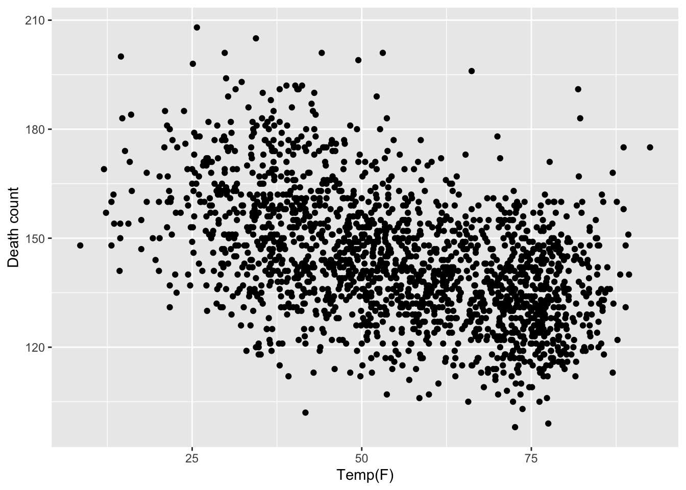
Come back to our mortality example

Consider the temperature and mortality analysis. Assume 40 equidistant knots and linear splines. The model is defined as:

\[ y_i = \beta_0 + \beta_1 x_i + \sum_{m=1}^{40} \beta_{1+m} (x_i - \kappa_m)_+, \]

where: - \(x_i\) represents the independent variable, - \(\kappa_m\) are the knot points, - \((x_i - \kappa_m)_+\) is the positive part function: \[ (x - \kappa)_+ = \begin{cases} x - \kappa, & \text{if } x > \kappa, \\ 0, & \text{if } x \leq \kappa. \end{cases} \]

We will penalize the coefficients \(\beta_{1+m}, \dots, \beta_{M+1}\) using the \(B\) matrix.

So \(\beta'B\beta = \sum_{m=1}^{40} \beta_{1+m}^2\)

knots <- seq(range(health$Temp)[1], range(health$Temp)[2], length.out = 40+2)
#place knots evenly on interior of the range of x

knots = knots[c(2:(length(knots)-1))]
X = cbind(rep(1, length(health$Temp)), health$Temp)

head(X)

     [,1] [,2]
[1,]    1 27.6
[2,]    1 25.1
[3,]    1 25.3
[4,]    1 29.8
[5,]    1 29.8
[6,]    1 33.9

for(i in 1:length(knots)){
  X = cbind(X, (health$Temp - knots[i]) * (health$Temp>knots[i]))
}

#Penalty matrix for regularization, 42 = number of coeffs
B = diag(42)

#Only spline terms for 3rd coefficient will be penalized
B[1,1] = 0
B[2,2] =0
dim(X)

[1] 1826   42

dim(B)

[1] 42 42

We now search through different values of \(\lambda\). For each \(\lambda\) we will:

• Calculate penalized \(\hat{\beta}\)

• Calculate \(\hat{\beta}'B\hat{\beta}\)

• Calculate fitted values \(\hat{Y} = X\hat{\beta}\)

• Calculate the GCV using the matrix \(X(X'X + \lambda B)^{-1} X'\)

We select the \(\lambda\) with the smallest GCV:

Y = health$alldeaths

lambda <- seq(0, 50, by = 5)

calc_gvc <- function(lambda, X, B){
beta = solve(t(X) %*% X + lambda*B) %*% t(X) %*% Y
H = X %*% solve(t(X) %*% X + lambda*B) %*% t(X)
Yhat = X %*% beta
GCV = mean((Y- Yhat)^2)/ (1-mean(diag(H)))^2
C = t(beta) %*% B %*% beta

return(GCV)
}

GCV <- rep(NA, length(lambda))
for(i in 1:length(lambda)){
  GCV[i] = calc_gvc(lambda = lambda[i], X, B)
}
GCV

 [1] 233.7743 231.8207 231.3576 231.1072 230.9433 230.8250 230.7344 230.6622
 [9] 230.6028 230.5528 230.5099

min(GCV)

[1] 230.5099

index = which(GCV == min(GCV))
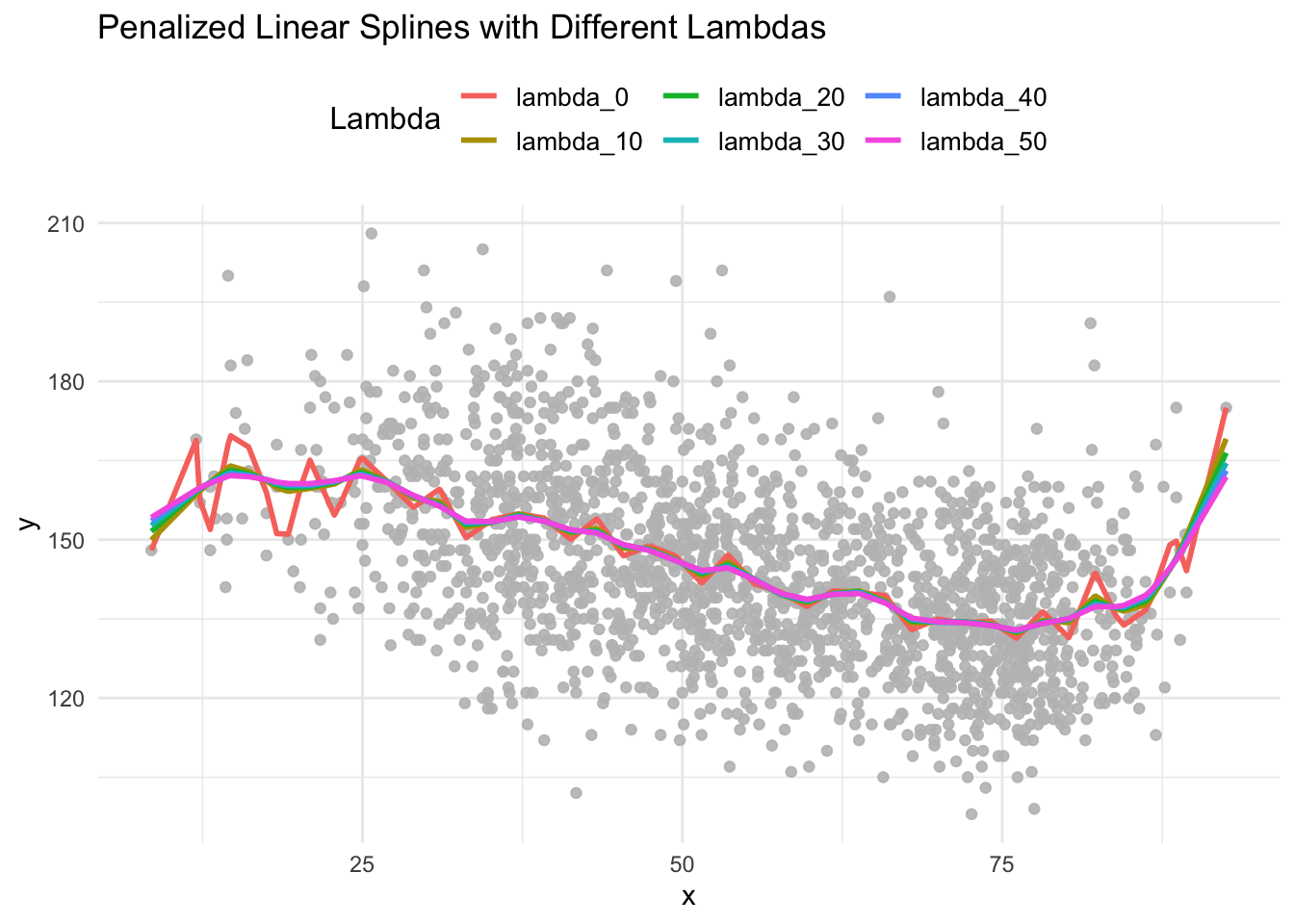
lambda[index]

[1] 50

Effect of Penalization

penalized_spline <- function(X, Y, lambda, B) {
# Create design matrix for linear splines
betahat = solve(t(X) %*% X + lambda*B) %*% t(X) %*% Y
H = X %*% solve(t(X) %*% X + lambda*B) %*% t(X)
Yhat = X %*% betahat
list_out <- list()
list_out[["Yhat"]] <- Yhat
list_out[["Betahat"]] <- betahat
return(list_out)
}

# Different lambda values to compare
lambdas <- seq(0, 50, by = 10)

# Create original data frame
original_data <- data.frame(x = health$Temp, y = health$alldeaths)


for(i in 1:length(lambdas)){
  res <- penalized_spline(X=X, Y=Y, B=B, lambda = lambdas[i])
  Yhat = res[["Yhat"]]
  original_data[[paste0("lambda_", lambdas[i])]] <- Yhat
}
# Convert wide to long
long_data <- original_data %>%
  pivot_longer(
    cols = starts_with("lambda_"),  # Select all lambda columns
    names_to = "lambda",           # Create a new column "lambda" for the column names
    values_to = "prediction"       # Create a new column "prediction" for the values
  )


# Plot using ggplot2
ggplot(long_data) +
  geom_point(aes(x = x, y = y), color = "grey", alpha = 0.3) +
  geom_line(aes(x = x, y = prediction[,1], color = lambda), linewidth = 1) +
  labs(
    title = "Penalized Linear Splines with Different Lambdas",
    x = "x",
    y = "y",
    color = "Lambda"
  ) +
  theme_minimal() +
  theme(
    legend.position = "top",
    legend.title = element_text(size = 12),
    legend.text = element_text(size = 10)
  )

Betahat_df <- array(NA, c(42, length(lambdas)))

# Compute Betahat for each lambda
for (i in 1:length(lambdas)) {
  res <- penalized_spline(X = X, Y = Y, B = B, lambda = lambdas[i])
  Betahat_df[, i] <- res[["Betahat"]]
}

# Convert array to dataframe
Betahat_df <- as.data.frame(Betahat_df)

# Name the columns after the lambda values
colnames(Betahat_df) <- paste0("lambda_", lambdas)

# Add a column for the indices of the Betahat values
Betahat_df$Coefficient <- 1:42

Betahat_long <- Betahat_df %>%
  pivot_longer(
    cols = starts_with("lambda_"),  # Select lambda columns
    names_to = "Lambda",            # Column for lambda values
    values_to = "Betahat"           # Column for Betahat values
  ) %>%
  mutate(Lambda = as.numeric(sub("lambda_", "", Lambda)))  # Clean lambda names



# Plot Betahat across different lambdas
ggplot(Betahat_long, aes(x = Coefficient, y = Betahat, color = as.factor(Lambda))) +
  geom_line(size = 1) +
  geom_point(size = 2, alpha = 0.8) +
  labs(
    title = "Penalized Linear Spline Coefficients Across Lambdas",
    x = "Coefficient Index",
    y = "Estimated Coefficient (Betahat)",
    color = "Lambda"
  ) +
  scale_color_brewer(palette = "Set1") +  # Optional: nice color palette
  theme_minimal() +
  theme(
    legend.position = "top",
    legend.title = element_text(size = 12),
    legend.text = element_text(size = 10),
    axis.title = element_text(size = 14),
    axis.text = element_text(size = 12)
  )

Warning: Using `size` aesthetic for lines was deprecated in ggplot2 3.4.0.
ℹ Please use `linewidth` instead.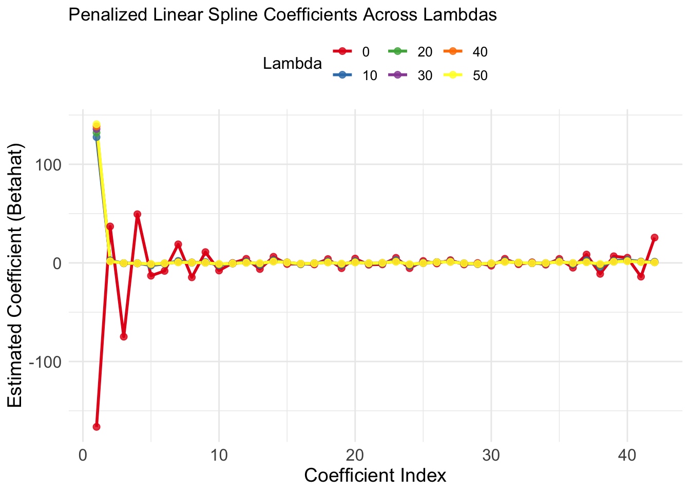

Key Takeaways from the Plot

• As \(\lambda\) increases:

  • Spline coefficients shrink, reducing their contribution to the model.

  • The model becomes smoother and less flexible, capturing broader trends but ignoring fine details.

• The intercept and linear terms (not penalized) changes significantly across \(\lambda\) because the penalty forces the model to rely more on the intercept when the spline coefficients are heavily penalized.

• The higher-index coefficients (spline terms) are the most affected, which is why you see their lines converge toward zero for larger \(\lambda\).

General Principle:

• \(\uparrow\) shrinkage \(\rightarrow\) \(\downarrow\) variance.
• \(\uparrow\) shrinkage \(\rightarrow\) \(\uparrow\) bias.

But how do we determine the level of shrinkage? i.e., how do we choose \(\lambda\)?

Generalized Cross-Validation Error

An approximation of leave-one-out cross-validation. Generalized Cross Validation Error is defined as

\[ \text{GCV}(\lambda) = \frac{1}{n} \frac{\sum_i (y_i -\hat{y})^2}{[1-\frac{1}{n} tr(H)]^2} = \frac{\text{RSS}}{\text{Effective degrees of freedom}} \]

Note that \(\hat{Y} =HY\) where \(H= X(X'X)^{-1}X'\) transform \(Y\rightarrow \hat{Y}\).

Now we can apply GCV to any prediction of \(Y\) that can be written in the form:

\[ \hat{Y} = SY \]

where \(S\) denotes a smoother matrix is generalization of the \(H\) matrix. In ridge regression \(S = X(X'X + \lambda B)^{-1} X\) (change from \(H\) matrix in OLS).

Each element is shrunk towards zero. We can define effective degrees of freedom \(df_{eff}\)

\[ df_{eff} = tr(S) \]

Important

Then GCV is defined as:

\[ GCV = \frac{1}{n} \frac{\sum_i (y_i -\hat{y})^2}{[1-\frac{1}{n} tr(S)]^2} \]

where \(S\) is the smoother matrix, and effective df is defined as \(tr(S)\).

# Simulate data for illustration
set.seed(123)
lambda_values <- seq(0.1, 100, length.out = 100)  # Range of lambda values
rss_values <- 500 / (lambda_values + 1) + rnorm(100, sd = 5)  # Simulate RSS
df_values <- 20 - 18 * (lambda_values / (lambda_values + 10))  # Effective df
gcv_values <- rss_values / (1 - df_values / 20)^2  # Compute GCV

# Create a dataframe for plotting
gcv_data <- data.frame(
  lambda = lambda_values,
  RSS = rss_values,
  df = df_values,
  GCV = gcv_values
)

# Find optimal lambda
optimal_lambda <- lambda_values[which.min(gcv_values)]
optimal_lambda

[1] 71.74545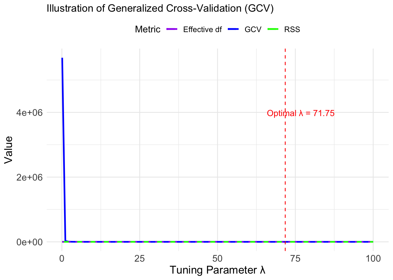

Residual Error Variance Estimate

We have two options:

\[ \hat{\sigma}^2 = \frac{\sum_{i=1}^n [y_i - \hat{g}(X_i)]^2}{n-df_{eff}} \] The above is a biased estimate. Some software gives the option to use:

\[ \hat{\sigma}^2_{unbiased} = \frac{\sum_{i=1}^n[y_i - \hat{g}(x_i)]^2}{n-2tr(S) + tr(SS')} \]

Lets derive \(Var(\hat{g}(x_i))\).

Confidence interval and prediction interval

Obtains point-wise confidence interval dervied from previous expression by plugging in \(\hat{\sigma}^2\).

Similarly, the variance for an unobserved point \(y_i^*\) with covariate\(x_i^*\) has variance:

\[ Var(y_i^*) = \sigma^2 + \sigma^2 x_i^* (X'X + \lambda B)^{-1} (X'X)(X'X + \lambda B)^{-1} x_i^* \]

[1] 3600

   user  system elapsed 
  3.779   0.011   3.797 

   user  system elapsed 
  0.044   0.013   0.056 

     [,1]
[1,] TRUE

[1] 15.11997

[1] 15.12668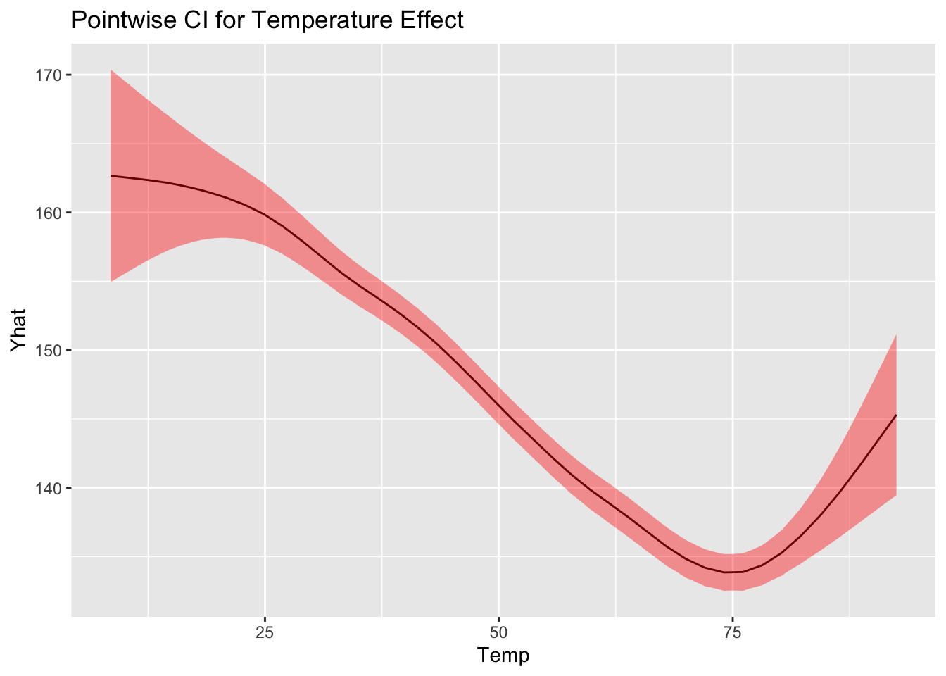

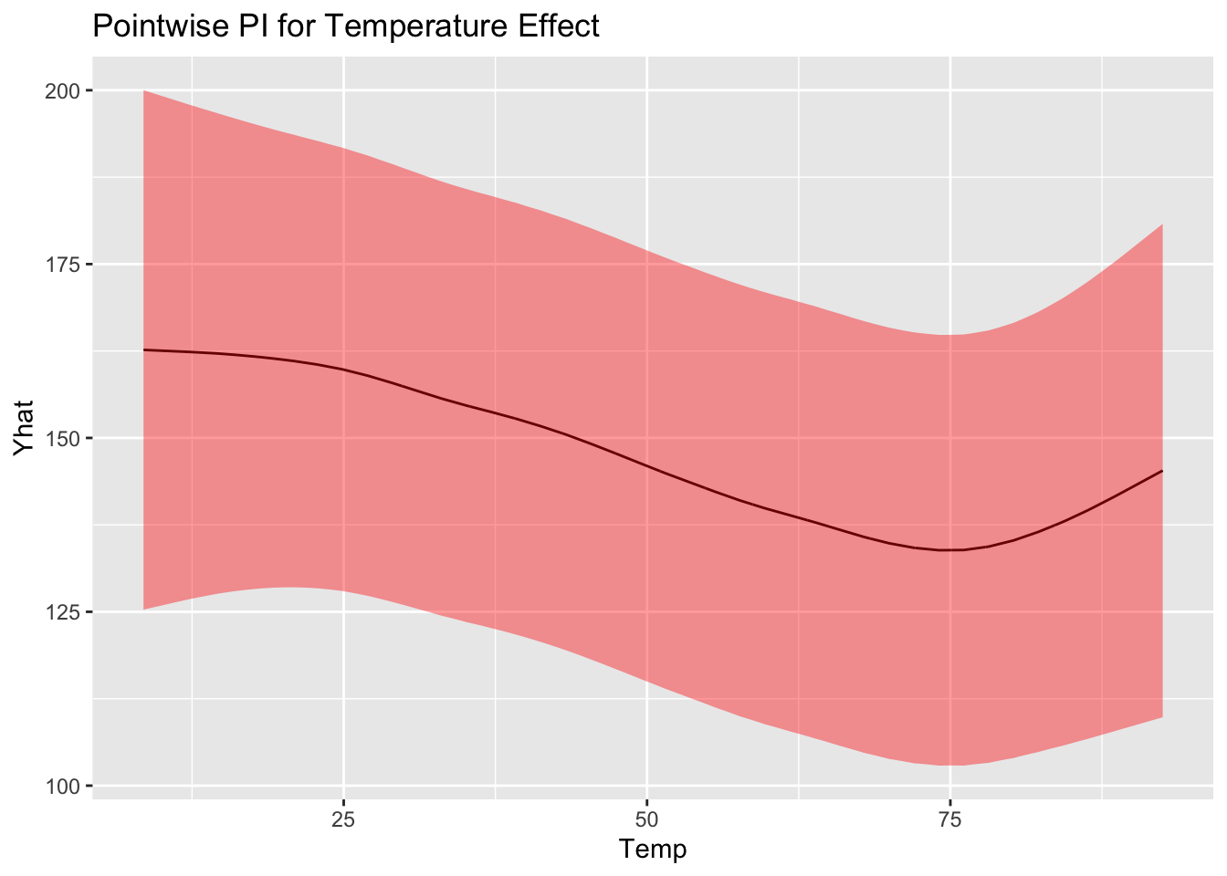
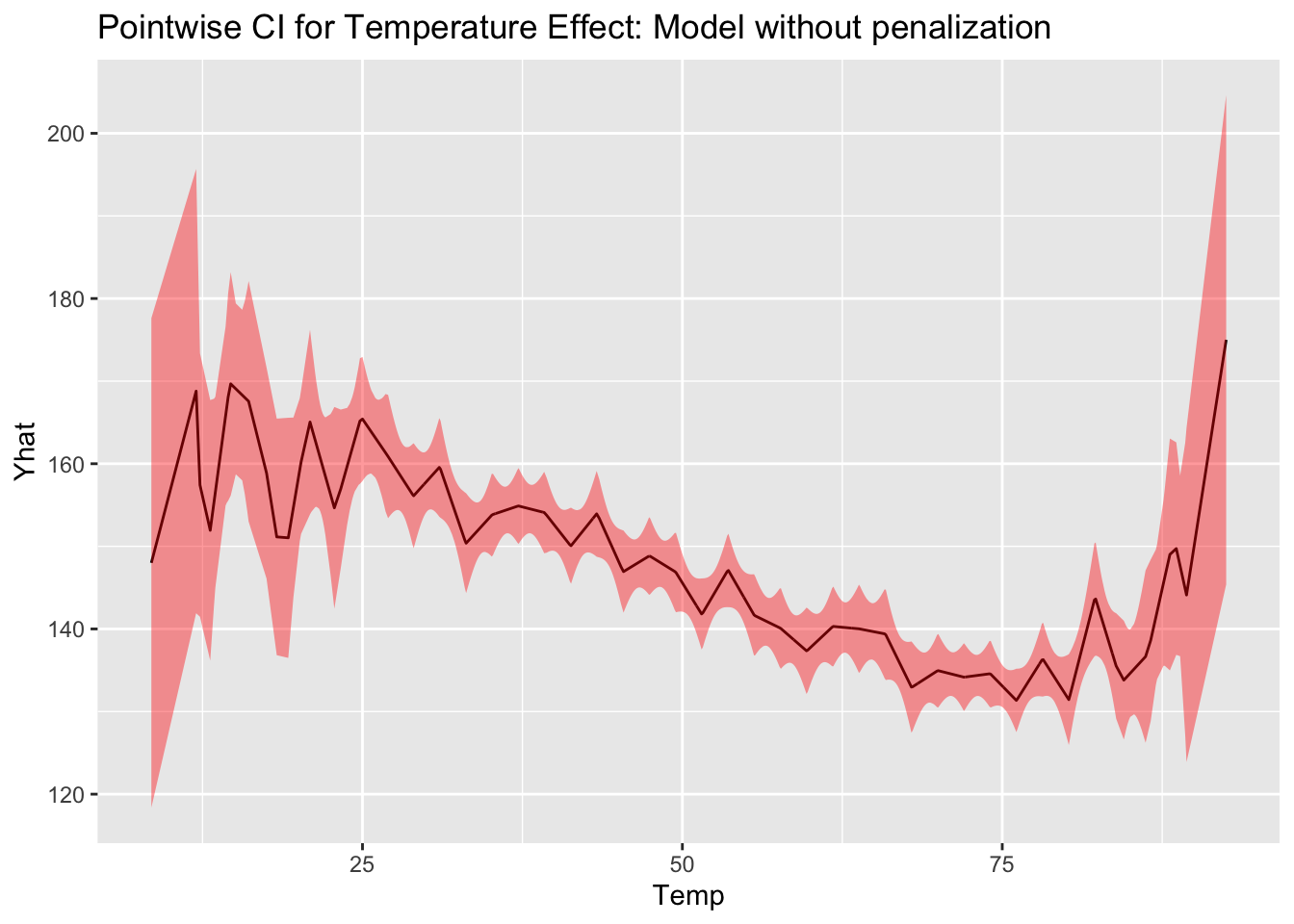
Smoothing Splines: other penalties

Important

• A smoothing spline is a statistical tool used to fit a smooth curve to a set of data points.
• Goal is to approximate an underlying function that explains the relationship between variables without assuming a specific functional form (like a linear or polynomial relationship).
  • Data Fitting: The smoothing spline minimizes the trade-off between model fit (through the sum of squared errors) and excessive curvature or smoothing.
  • Smoothness: The curve generated by a smoothing spline is smooth (no discontinuities) while avoiding overfitting.
  • Regularization: Smoothing splines are regularized, i.e., they include a penalty for too much curvature in the fitted curve, controlling the degree of smoothness. This penalty is determined by a smoothing parameter, often denoted by \(\lambda\).In summary, we add a “roughness” penalty to encourage smoothness:

\[ \hat{g}(x) = \underset{g \in G}{argmin}\{Y-g(X)\}'\{Y-g(X)\} + \lambda \underset{\text{roughness penalty}}{\int_a^b (g''(X\beta))^2dx\}} \]

• Note the 1st derivatives are not penalized
• 2nd part uses the squared 2nd-derivative that is a good measure of roughness.
• Shrinks coefficients in a cubic polynomial, causing function to change less quickly. (ie large penalties reduce wiggliness).
• \(\lambda\) controls trade-off between the two terms. Small \(\lambda\) prioritizes closeness to data vs. large \(\lambda\) prioritizes smoothness.

Smoothing Splines with mgcv in R

The mgcv (Mixed GAM Computation Vehicle) package in R provides the gam() function to fit a wide variety of smoothing splines with automatic smoothing parameter selection. Throughout this class, we will explore different options available in mgcv.

Below are some key default settings:

Default Options:

1. Basis Functions
   Default: Thin plate regression spline.

2. Basis Dimension
   Default: \(k = 10\) with one constraint \(\hat{g}(x_i) = 0\), making the maximum effective degrees of freedom (\(\text{edf}\)) equal to 9. The minimum \(\text{edf}\) is 1 (unpenalized linear term).

   • If \(\text{edf} = 1\), the results are nearly equivalent to lm().

3. Selection Methods
   Default: Generalized Cross Validation (GCV).

4. Family
   Default: Gaussian.

5. Standard Error Computation
   Default: Bayesian.

• Flexibility: GAMs can handle multiple predictors, each with potentially different non-linear relationships to the response. These relationships are modeled using smoothing splines, thin plate splines, or other basis functions.

• Automatic Smoothing: GAM frameworks like mgcv use methods such as Generalized Cross-Validation (GCV) or Restricted Maximum Likelihood (REML) to automatically choose smoothing parameters for each term.

Comparing Smoothing Splines to GAMs

Feature	Smoothing Splines	Generalized Additive Models (GAMs)
Scope	Single predictor	Multiple predictors
Additive Structure	No	Yes
Link Function	Not applicable (linear)	Supports different link functions (e.g., log, logit)
Smoothing	Single penalty term	Separate penalties for each predictor’s smooth term
Software	Standalone or integrated	Built into GAM frameworks like mgcv

Relationship

• GAMs often use smoothing splines (or similar smoothers) as the functional form for each predictor in the additive model. For example, the gam() function in mgcv allows specifying smooth terms like s(x) or te(x, z), which are internally fitted using basis functions, including smoothing splines.

Coming back to our example: Temperature Effect on Mortality

library (mgcv)

Loading required package: nlme

Attaching package: 'nlme'

The following object is masked from 'package:dplyr':

    collapse

This is mgcv 1.8-42. For overview type 'help("mgcv-package")'.

fit1 = gam(alldeaths~s(Temp), data= health)
summary(fit1)

Family: gaussian 
Link function: identity 

Formula:
alldeaths ~ s(Temp)

Parametric coefficients:
            Estimate Std. Error t value Pr(>|t|)    
(Intercept) 143.9168     0.3538   406.8   <2e-16 ***
---
Signif. codes:  0 '***' 0.001 '**' 0.01 '*' 0.05 '.' 0.1 ' ' 1

Approximate significance of smooth terms:
          edf Ref.df     F p-value    
s(Temp) 6.026    7.2 80.62  <2e-16 ***
---
Signif. codes:  0 '***' 0.001 '**' 0.01 '*' 0.05 '.' 0.1 ' ' 1

R-sq.(adj) =  0.241   Deviance explained = 24.3%
GCV = 229.47  Scale est. = 228.58    n = 1826

Interpretation:

• Parametric Coefficients:
  • Intercept:
    • Estimate = 143.92
      
    • Standard Error = 0.35
      
    • t-value = 406.8
      
    • p-value = < 2e-16 (***)
• Smooth Terms:
  • s(Temp):
    • Estimated Degrees of Freedom (edf) = 6.03. Relationship is non-linear.
    • Reference Degrees of Freedom (Ref.df) = 7.2
      
    • F-value = 80.62
      
    • p-value = < 2e-16 (***). Association between temp and deaths is significant.
• Model Fit:
  • Adjusted ( R^2 ) = 0.241 (24.1% of variance explained)
    
  • Deviance Explained = 24.3%
    
  • Generalized Cross-Validation (GCV) Score = 229.47.
  • Scale Estimate = 228.58
    
  • Sample Size ((n)) = 1826

Checking GAMs

mgcv::gam.check(fit1)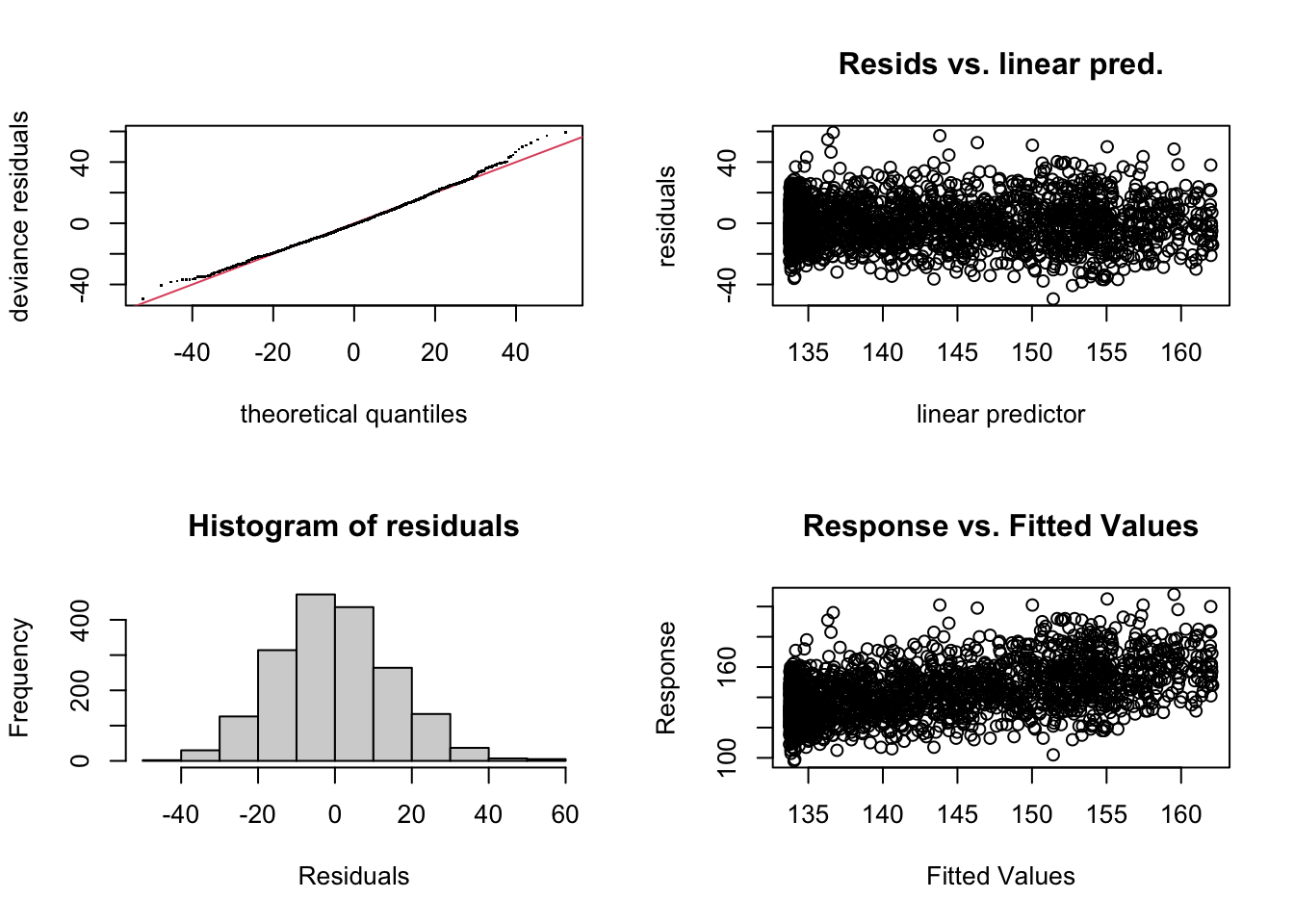

Method: GCV   Optimizer: magic
Smoothing parameter selection converged after 5 iterations.
The RMS GCV score gradient at convergence was 7.241958e-05 .
The Hessian was positive definite.
Model rank =  10 / 10 

Basis dimension (k) checking results. Low p-value (k-index<1) may
indicate that k is too low, especially if edf is close to k'.

          k'  edf k-index p-value
s(Temp) 9.00 6.03    1.02    0.86

The default \(k\) for GAMs is \(k=10\). Increase \(k=40\), run the same model as above and compare the GCVs to find best model fit.