Module 1: Multiple Linear Regression Review

Reading

• Review matrix algebra, see materials in Module 0 on Canvas. For more advanced review see The Matrix Cookbook.
• Review notes from Applied Linear Regression (BIOS 509)

  • Other useful materials:

    

Concepts

• Linear regression model in matrix notation.

• Inference for regression coefficient estimates, expected values, and predictions.

• Dummy variables.

• Effect modification, interactions, and confounding.

Acknowledgements

• Lecture notes are build upon materials from Prof. Benjamin Risk and Howard Chang.

Motivating Example

We are interested in the maternal traits associated with children’s cognitive test scores at age 3. Using data from a survey of adult American women and their children from the National Longitudinal Survey of Youth.

Variables:

• score: cognitive test score at age 3.

• age: maternal age at delivery

• edu: maternal education (1) less than high school, (2) high school, (3) some college, (4) college and above.

library(readr)
dat <- read_csv("data/testscore.csv")

Rows: 400 Columns: 3
── Column specification ────────────────────────────────────────────────────────
Delimiter: ","
dbl (3): score, edu, age

ℹ Use `spec()` to retrieve the full column specification for this data.
ℹ Specify the column types or set `show_col_types = FALSE` to quiet this message.

head(dat)

# A tibble: 6 × 3
  score   edu   age
  <dbl> <dbl> <dbl>
1   120     2    21
2    89     1    17
3    78     2    19
4    42     1    20
5   115     4    26
6    97     1    20

str(dat)

spc_tbl_ [400 × 3] (S3: spec_tbl_df/tbl_df/tbl/data.frame)
 $ score: num [1:400] 120 89 78 42 115 97 94 68 103 94 ...
 $ edu  : num [1:400] 2 1 2 1 4 1 1 2 3 3 ...
 $ age  : num [1:400] 21 17 19 20 26 20 20 24 19 24 ...
 - attr(*, "spec")=
  .. cols(
  ..   score = col_double(),
  ..   edu = col_double(),
  ..   age = col_double()
  .. )
 - attr(*, "problems")=<externalptr> 

summary(dat$score)

   Min. 1st Qu.  Median    Mean 3rd Qu.    Max. 
  20.00   74.00   90.00   86.93  102.00  144.00 

table(dat$edu)

  1   2   3   4 
 85 212  76  27 

summary(dat$age)

   Min. 1st Qu.  Median    Mean 3rd Qu.    Max. 
  17.00   21.00   23.00   22.79   25.00   29.00 

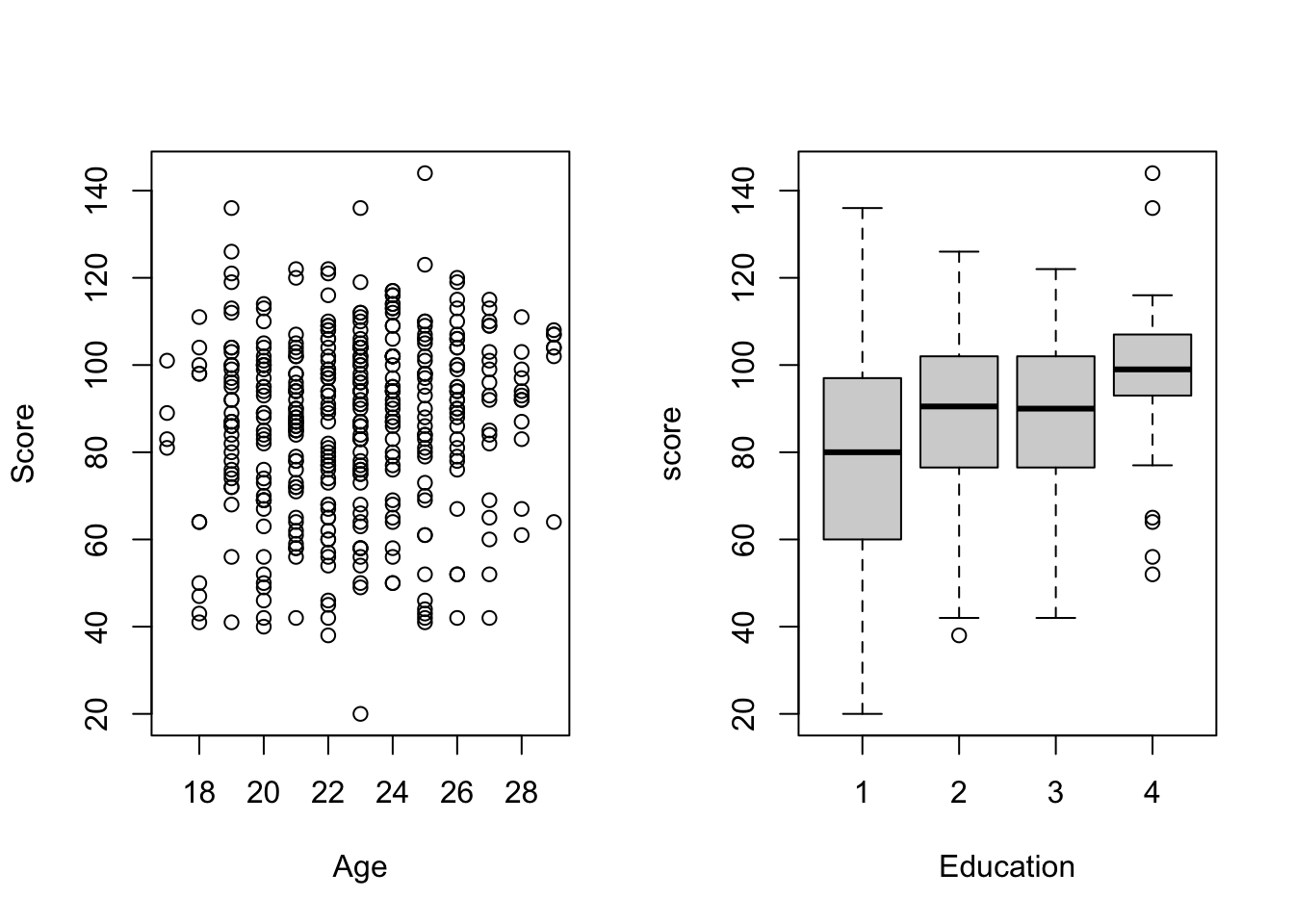
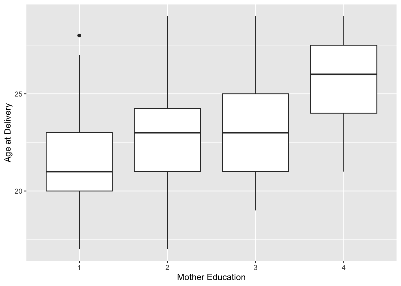
par(mfrow = c(1,2))
plot(score ~ age, data = dat, xlab = "Age", ylab = "Score")
boxplot(score ~ edu, xlab = "Education", data = dat)

Simple Linear Regression

Linear regression is a method that summarizes how the average values of a numerical outcome variable vary over subpopulations defined by linear functions of predictors. Two goals of linear regression:

1. Prediction of outcome values given fixed predictor values.

2. Assessment of impact of predictors on the outcome (Estimation).

Let $y_i$ denote the test score for a given child $i$. $ag{e}_i$ denotes the corresponding maternal age at delivery for mom $i$ corresponding to child $i$, and ${ϵ}_i$ denotes the error term. We will consider the following linear model:

$$\begin{array}{}\text{(1)}& y_i={\beta }_0+{\beta }_1\cdot ag{e}_i+{ϵ}_i,i=1,2,3,...,400\end{array}$$

We can write Eq. 1 in matrix form by stacking observations by row:

$$\begin{array}{rl}\mathbf{Y}& =\left[\begin{array}{c}{y}_1\\ y_2\\ ⋮\\ y_n\end{array}\right]=\left[\begin{array}{c}{\beta }_0+{\beta }_1{x}_1\\ {\beta }_0+{\beta }_1{x}_2\\ ⋮\\ {\beta }_0+{\beta }_1{x}_n\end{array}\right]+\left[\begin{array}{c}{ϵ}_1\\ {ϵ}_2\\ ⋮\\ {ϵ}_n\end{array}\right]\\ & =\left[\begin{array}{cc}1& x_1\\ 1& x_2\\ ⋮\\ 1& x_n\end{array}\right]\left[\begin{array}{c}{\beta }_0\\ {\beta }_1\end{array}\right]+\left[\begin{array}{c}{ϵ}_1\\ {ϵ}_2\\ ⋮\\ {ϵ}_n\end{array}\right]\\ & =\mathbf{X}\beta \mathbf{+}ϵ\end{array}$$

In-class exercise

Define the different components $(Y,X,\beta ,ϵ)$.

What is the expected value of $\mathbf{Y}$?

What is the variance of $\mathbf{Y}$?

What is the covariance of $cov(y_i,y_j)$?

Assumptions of the above model

• $y_i$ is a linear function of $ag{e}_i$, i.e, $E(\mathbf{Y})=\mathbf{X}\beta =\mathbf{Age}\beta$ is linear.

• ${\beta }_0=$ the test score for a child born of a mother at age=0 (not meaningful!)

• ${\beta }_1=$ increase in test score associated with one year increase in maternal age.

• $E({ϵ}_i)=0$ Expectation of the errors in zero.

Least Squares Solution

Our aim is to find estimates of ${\beta }_0$ and ${\beta }_1$ that “best” fit the data, but what does “best” mean?

We seek $({\hat{\beta }}_0,{\hat{\beta }}_1)$ that minimizes a loss function.

Our approach is to minimize the sum of squared differences between $\mathbf{Y}$ and $\hat{Y}=\mathbf{X}\hat{\beta }$, i.e., this defines the differences between $\mathbf{Y}$ and the predicted value $\hat{Y}$ based on a fixed set of ${\beta }^{\prime }s$.

Theorem

If $\mathbf{Y}=\mathbf{X}\beta +ϵ$ then the value of $\hat{\beta }$ that minimizes $(\mathbf{Y}\mathbf{-}\hat{\mathbf{Y}}{)}^T(\mathbf{Y}\mathbf{-}\hat{\mathbf{Y}})$ is $\hat{\beta }=(X^{\prime }X{)}^{-1}{X}^{\prime }y$.

• $\hat{\mathbf{Y}}=\mathbf{X}\hat{\beta }$ is the fitted (predicted) value.

• $\widehat{ϵ}-\mathbf{Y}=\mathbf{X}\hat{\beta }$ defines the residual error.

In-class exercise

Let’s show this!

• For OLS, we have a nice closed-form solution.

• Other loss functions or models often require iterative optimization routines.

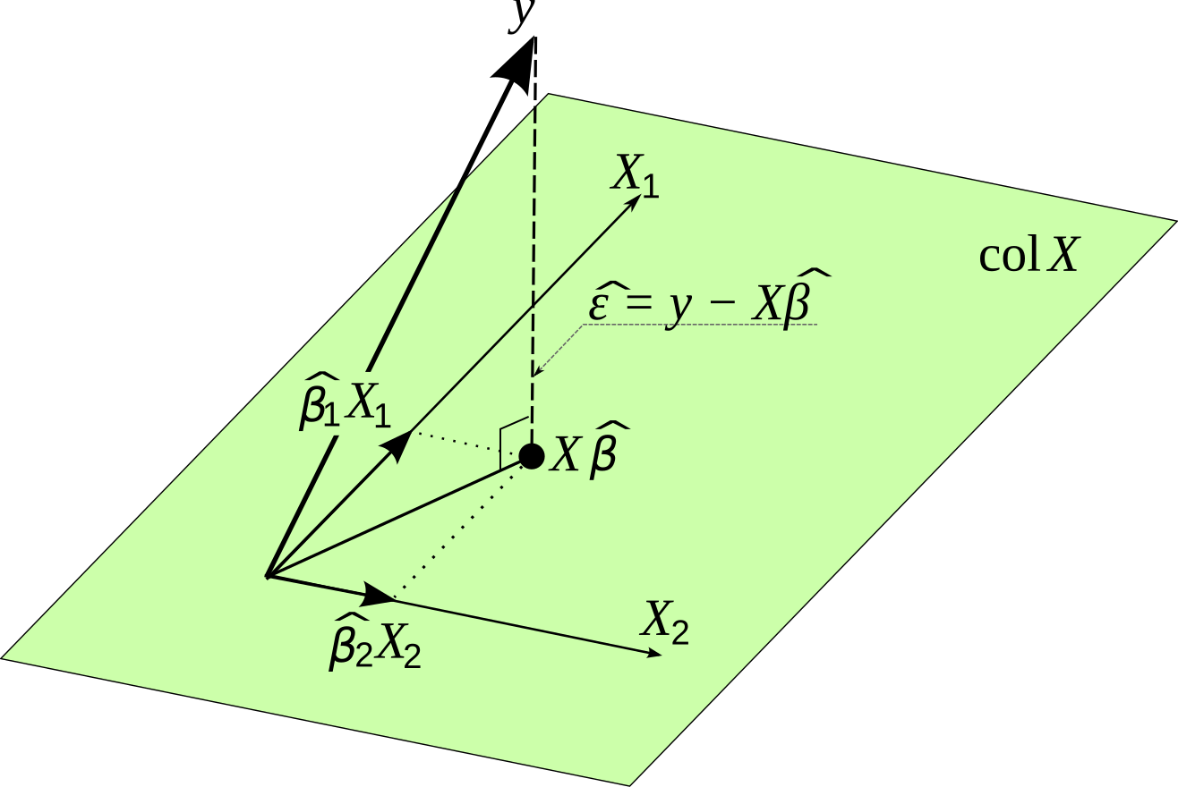
Geometric Interpretation of the OLS estimate

The fitted values $\hat{y}$ are a linear transformation of $y$. We $y$ in real space is projected on $\hat{y}$ is model space.

• The HAT matrix is defined as $\mathbf{H}=\mathbf{X}\mathbf{(}{\mathbf{X}}^{\mathbf{T}}\mathbf{X}{\mathbf{)}}^{\mathbf{-}\mathbf{1}}{\mathbf{X}}^{\mathbf{T}}$. It is a projection matrix that projects $y$ to $\hat{y}$.

  $$\begin{array}{rl}\hat{\mathbf{y}}& =\mathbf{X}\hat{\beta }\\ & =\mathbf{X}\mathbf{(}{\mathbf{X}}^{\prime }\mathbf{X}{\mathbf{)}}^{\mathbf{-}\mathbf{1}}{\mathbf{X}}^{\prime }\mathbf{y}\end{array}$$

• The projection matrix is idempotent, i.e., $HH=H$.

• The trace of the projection matrix is the number of covariates plus intercept, i.e, $tr(H)=p$.

• $\hat{\mathbf{Y}}$ and $\widehat{ϵ}$ are independent, i.e., orthogonal (perpendicular in model space).

A geometrical interpretation of least squares.

Properties of the OLS Estimator $\hat{\beta }$

1. If $E(Y)=X\beta$ then $\hat{\beta }$ is unbiased for $\beta$.

2. $\hat{\beta }$ is consistent estimation of $\beta$ under very general assumptions, i.e., $li{m}_{n\to \mathrm{\infty }}P(|\hat{\beta }-\beta |>ϵ)=0$.

3. $\hat{\mathbf{Y}}$ is an unbiased estimator of the mean trend $\mathbf{X}\beta$.

4. If $cov(y)={\sigma }^{2}I$, the covariance of the estimator $cov(\hat{\beta })={\sigma }^2(X^{\prime }X{)}^{-1}$.

In-class exercise

Find the $cov(\hat{\beta })$.

Gauss-Markov Theorem

• $\mathbf{Y}=\mathbf{X}\beta +ϵ$

• $E(ϵ)=0$ and $cov(ϵ)={\sigma }^{2}I$

• $var(\hat{\beta })={\sigma }^2(X^{\prime }X{)}^{-1}$

• $\hat{\beta }$ is the best (minimum variance) unbiased estimator (BLUE) for $\beta$.

OLS Calculation in R

X = cbind(1, dat$age) #Design Matrix
Y = dat$score #Response/Outcome Vector
beta = solve( t(X) %*% X) %*% t(X) %*% Y
beta

           [,1]
[1,] 67.7826813
[2,]  0.8402729

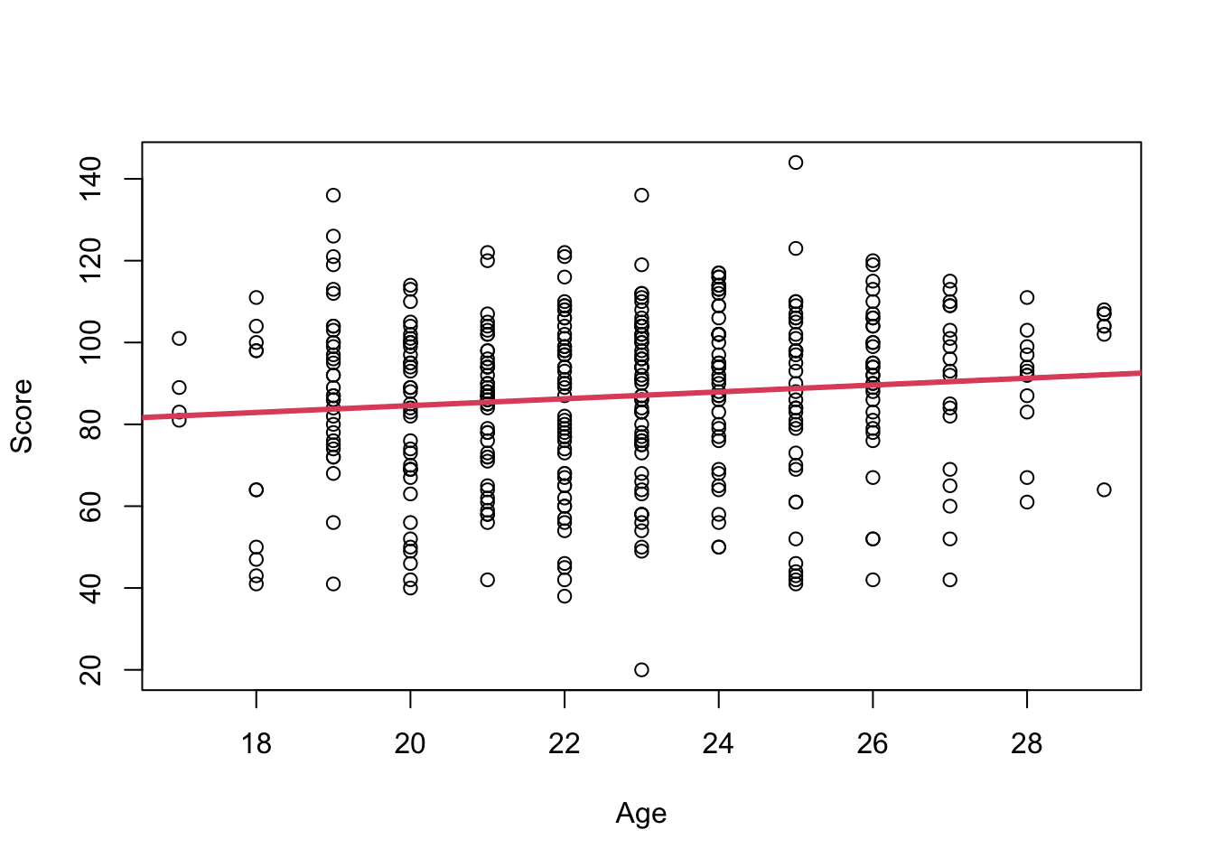
plot(score ~ age, data = dat, xlab = "Age", ylab = "Score")
abline(beta, lwd = 3, col = 2)

Summary I

What is the model?	In simple linear regression, we regress a vector of outcomes $Y$ values on a vector of predictor values $X$ with: $Y=X\beta +ϵ$ $\beta$ is a $2\times 1$ vector of regression coefficients: (1) the intercept ${\beta }_0$ , and (2) the covariate coefficient ${\beta }_1$.
Model Assumptions	$E(ϵ)=0$ $Var(ϵ)={\sigma }^2$ global variance $y$ is a linear function of $x$ $y\perp ϵ$ orthogonality $=$ independence
Least Squares Solution	$\hat{\beta }=(X^{\prime }X{)}^{-1}{X}^{\prime }y$ is the best (smallest variance) linear unbiased estimator of the true $\beta$ $E(\hat{\beta })=\beta$ and $cov(\hat{\beta })={\sigma }^2(X^{\prime }X{)}^{-1}$ The HAT matrix $X(X^{\prime }X{)}^{-1}{X}^{\prime }$ is a projection matrix which projects $y$ to $\hat{y}=X\hat{\beta }$
Interpretation	${\beta }_0$ the global value of $E(Y)$ when $X=0$ ${\beta }_1$ the global value of the change of $Y$ for every one unit change of $X$ ${\sigma }^2$ captures the total variance across all observations

Statistical Linear Regression & Inference

The relation between OLS, Normality, and Maximum Likelihood

So far, we have not discussed the distribution of the errors. For OLS we did not need to make any distributional assumption. For inference, let’s now assume

$$y_i={\beta }_0+{\beta }_{1}ag{e}_i+{ϵ}_i,i=1,...,400$$ where $ϵ\stackrel{iid}{\sim }N(0,{\sigma }^2)$.

What does i.i.d mean? identically and independently distributed. This implies the following model:

• $y_i$ is normally distributed.

• This parametrization is equal to

  $$y_i\sim N({\beta }_0+{\beta }_1{x}_i,{\sigma }^2)$$.

• where ${\beta }_0+{\beta }_1{x}_i$ captures the trend

• where ${\sigma }^2$ captures the variability (uncertainty) around the trend. It is constant, i.e., the same across all observations.

• In matrix form: $\mathbf{Y}\sim N(\mathbf{X}\beta ,\mathrm{\Sigma })$ where $\mathrm{\Sigma }={\sigma }^{2}I$.

• ${\sigma }^2$ is unkown!

The Maximum Likelihood

The likelihood of the normal distribution is given by

$$L(\beta ,{\sigma }^2,y)=(2\pi {\sigma }^2{)}^{-n/2}exp(\frac{-1}{2{\sigma }^2}(Y-X\beta {)}^{\prime }(Y-X\beta ))$$

Taking the log of the likelihood, we get:

$$l(\beta ,{\sigma }^2,y)=\frac{-n}{2}log(2\pi {\sigma }^2)-\frac{1}{2{\sigma }^2}(Y-X\beta {)}^{\prime }(Y-X\beta )$$

To find Maximum Likelihood Estimators we take partial derivatives and set the equal to zero to find the estimators that maximize the log-likelihood.

What do we get?

• ${\hat{\beta }}_{MLE}=(X^{\prime }X{)}^{-1}{X}^{\prime }y$ so ${\hat{\beta }}_{MLE}={\hat{\beta }}_{OLS}$ under normality.

• ${\hat{\sigma }}_{MLE}^2=\frac{1}{n}(Y-X\hat{\beta }{)}^{\prime }(Y-X\hat{\beta })$.

• $E({\hat{\sigma }}_{MLE}^2)\ne {\sigma }^2$ so it is NOT unbiased.

• An unbiased estimator for ${\sigma }^2$ is given by $s^2=\frac{1}{n-p}(Y-X\beta {)}^{\prime }(Y-X\beta )$.

Summary of OLS vs. MLE approaches

	OLS	MLE
Distributional assumption	NONE	Normal $Y\sim N(X\beta ,{\sigma }^{2}I)$
Estimator $\hat{\beta }$	$(X^{\prime }X{)}^{-1}{X}^{\prime }y$	$(X^{\prime }X{)}^{-1}{X}^{\prime }y$
$cov(\hat{\beta })$	${\sigma }^2(X^{\prime }X{)}^{-1}$	${\sigma }^2(X^{\prime }X{)}^{-1}$
Estimator ${\hat{\sigma }}^2$	Cannot get	$\frac{1}{n}(Y-X\hat{\beta }{)}^{\prime }(Y-X\hat{\beta })$ is biased

Residual Error

Above we determined that the unbiased estimator of ${\sigma }^2$ is $\frac{1}{n-p}(Y-X\hat{\beta }{)}^{\prime }(Y-X\hat{\beta })$.

library(ggplot2)

#Here p = 2
fit = lm(score ~ age, data = dat)

summary(fit)

Call:
lm(formula = score ~ age, data = dat)

Residuals:
    Min      1Q  Median      3Q     Max 
-67.109 -11.798   2.971  14.860  55.210 

Coefficients:
            Estimate Std. Error t value Pr(>|t|)    
(Intercept)  67.7827     8.6880   7.802 5.42e-14 ***
age           0.8403     0.3786   2.219    0.027 *  
---
Signif. codes:  0 '***' 0.001 '**' 0.01 '*' 0.05 '.' 0.1 ' ' 1

Residual standard error: 20.34 on 398 degrees of freedom
Multiple R-squared:  0.01223,   Adjusted R-squared:  0.009743 
F-statistic: 4.926 on 1 and 398 DF,  p-value: 0.02702

#Can we confirm this manually
yhat = fit$fitted.values #Predicted Values
y = dat$score #Observed Values
N = length(y)
P=2 #number columns in design matrix
sq_error = (y-yhat)^2 #Squared errors
sigma_squared_est <- sum(sq_error)/(N-P) #Unbiased est of the variance
sigma_est = sqrt(sigma_squared_est) #Unbiased est of the std. error
sigma_est

[1] 20.34027

#Include 95% confidence intervals in your summary

confidence_intervals <- predict(
  fit, 
  interval = "confidence", 
  level = 0.95
)
confidence_intervals[1:3,]

       fit      lwr      upr
1 85.42841 83.02579 87.83104
2 82.06732 77.31656 86.81808
3 83.74787 80.29024 87.20549

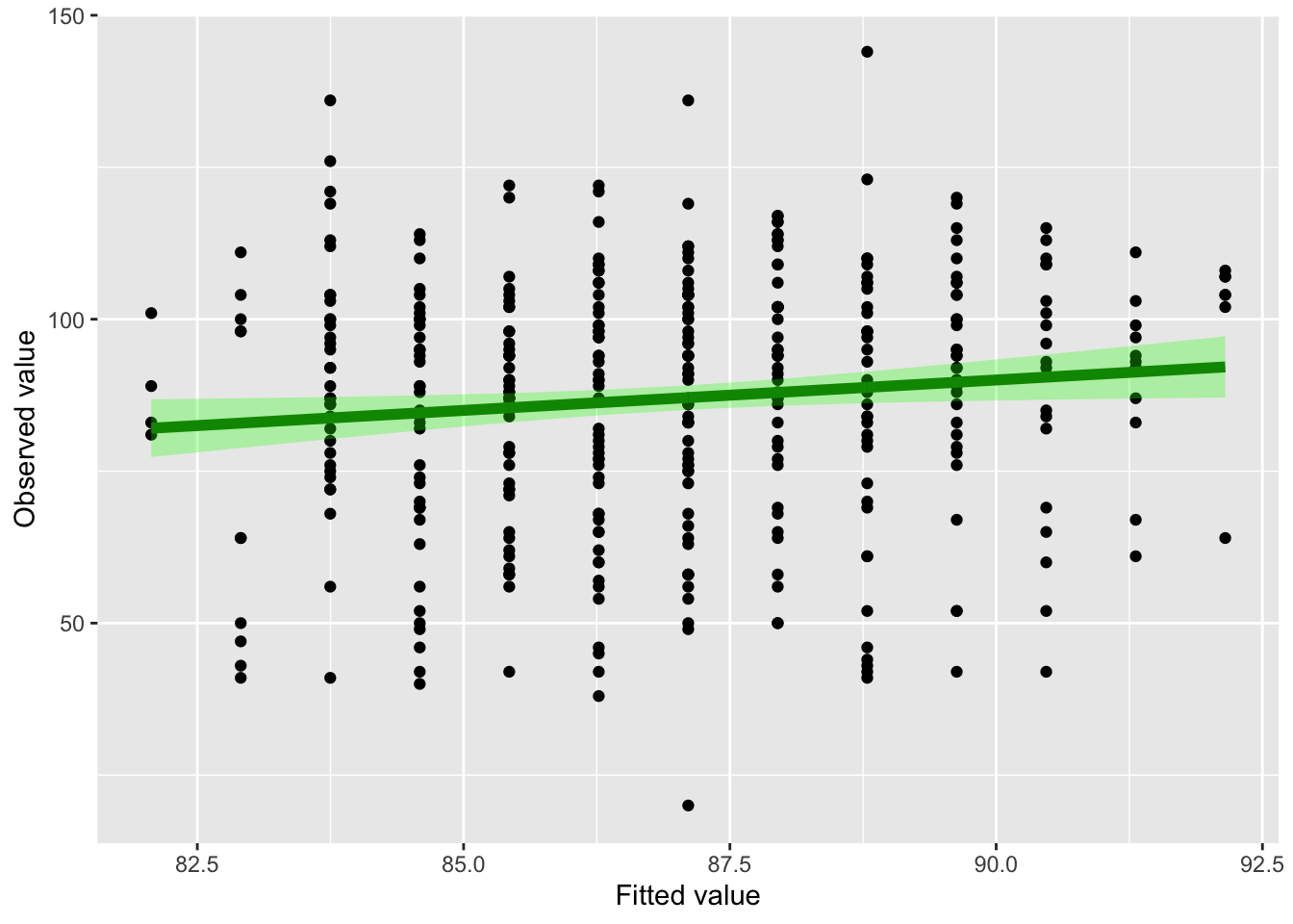
est <- fit$coefficients[1] + fit$coefficients[2] * dat$age

#Now add the 95% confidence intervals surrounding the fitted values
plot_data <- data.frame(dat$age, dat$score, confidence_intervals, est)

ggplot(plot_data) +
  geom_point(aes(fit, dat.score)) +
  geom_line(aes(fit,est), col = "darkgreen", lwd=2) +
  geom_ribbon(aes(x=fit, ymin =lwr, ymax = upr ), fill = "green", alpha = 0.3) +
  labs(x = "Fitted value", y = "Observed value")

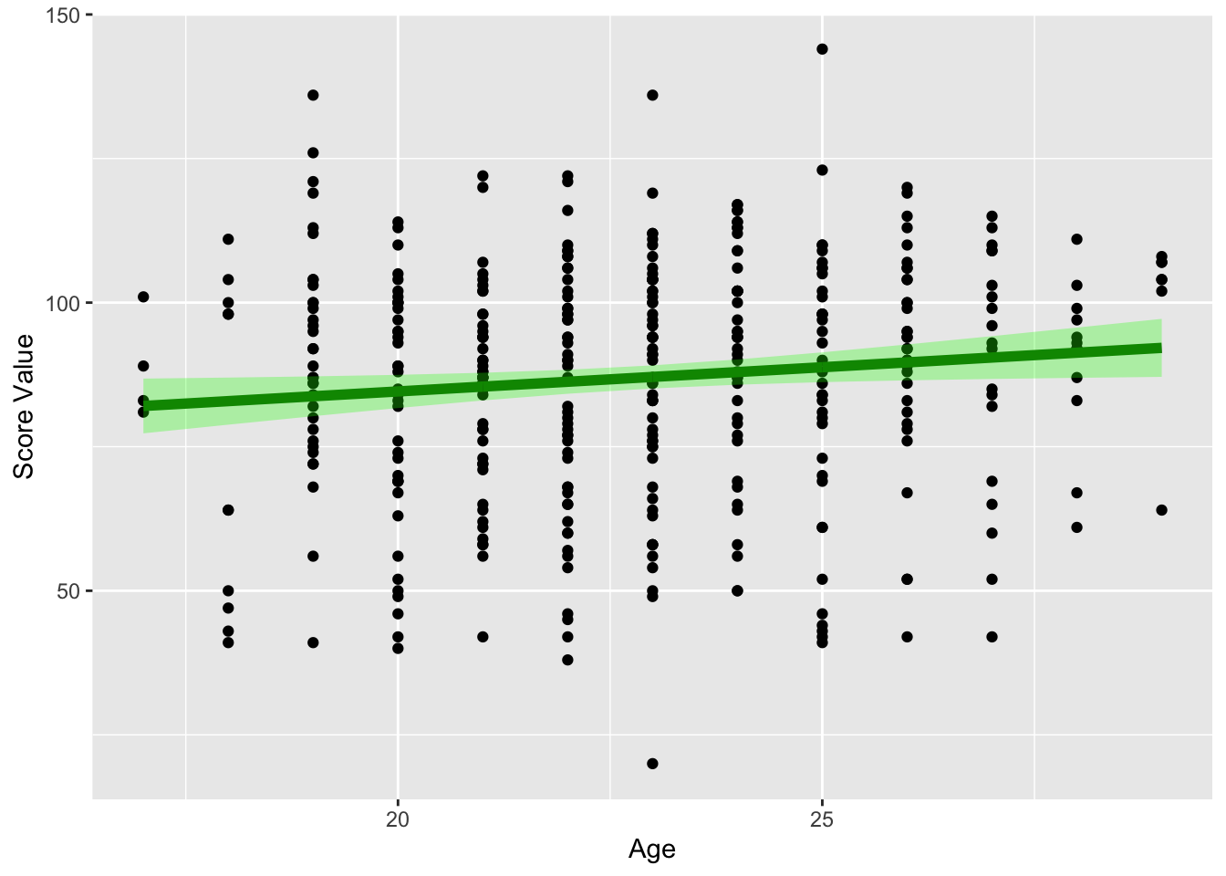
ggplot(plot_data) +
  geom_point(aes(dat.age, dat.score)) +
  geom_line(aes(dat.age,est), col = "darkgreen", lwd=2) +
  geom_ribbon(aes(x=dat.age, ymin =lwr, ymax = upr ), fill = "green", alpha = 0.3) +
  labs(x = "Age", y = "Score Value")

Model Interpretation

fit = lm(score ~ age, data = dat)
summary(fit)

Call:
lm(formula = score ~ age, data = dat)

Residuals:
    Min      1Q  Median      3Q     Max 
-67.109 -11.798   2.971  14.860  55.210 

Coefficients:
            Estimate Std. Error t value Pr(>|t|)    
(Intercept)  67.7827     8.6880   7.802 5.42e-14 ***
age           0.8403     0.3786   2.219    0.027 *  
---
Signif. codes:  0 '***' 0.001 '**' 0.01 '*' 0.05 '.' 0.1 ' ' 1

Residual standard error: 20.34 on 398 degrees of freedom
Multiple R-squared:  0.01223,   Adjusted R-squared:  0.009743 
F-statistic: 4.926 on 1 and 398 DF,  p-value: 0.02702

Interpretation: A one year increase in mother’s age at delivery was associated with a X (95%CI = ) increase in the child’s average test score, where test score was measured at age 3. Th association was statistically signifianct at a type I error rate of 0.05.

There was considerable heterogeneity in test scores $(\hat{\sigma }=20.34)$. Therefore, the regression model does not predict individual test scores well $(R^2=0.012)$. 1.2% of variances is explained by mother’s age.

Prediction Interval for a New Observation

Let ${\tilde{y}}_i$ be a new observation with covariate value $ag{e}_i$. How can you obtain its uncertainty? We want to capture the uncertainty in our predicted estimate of the expected value ${\hat{y}}_i=X\hat{\beta }$ PLUS the uncertainty due to measurement error ${ϵ}_i$.

$${\tilde{y}}_i={\hat{\beta }}_0+{\hat{\beta }}_{1}ag{e}_i+{ϵ}_i,{ϵ}_i\sim N(0,{\sigma }^2)$$

The total uncertainty surrounding the predicted value ${\tilde{y}}_i$ can be broken down as the sum of two components.

Taking the variance of Equation XX.

$$Var({\tilde{y}}_i)=Var({\hat{\beta }}_0+{\hat{\beta }}_{1}ag{e}_i)+Var({ϵ}_i)$$

• We know the first term on the right, $Var(\hat{\beta })={\sigma }^2(X^{\prime }X{)}^{-1}$ and so $Var(X\hat{\beta })={\sigma }^2(x_i^{{}^{\prime }}(X^{\prime }X{)}^{-1}{x}_i)$.
• We know the variance of the error term $Var({ϵ}_i)={\sigma }^2$.

We plug in our estimators to get the predicted variance

$${\tilde{\sigma }}^2=Var({\tilde{y}}_i)={\hat{\sigma }}^2{x}_i^T(X^{T}X{)}^{-1}{x}_i+{\hat{\sigma }}^2$$

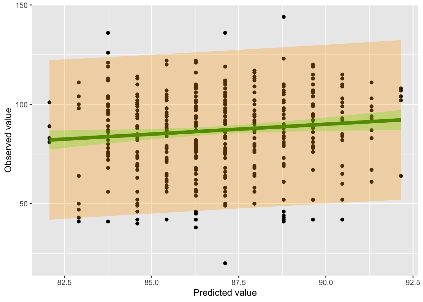
From this derivation we can see that ${\tilde{\sigma }}^2\ge {\hat{\sigma }}^2$. So the 95% prediction interval is going to be wider than the 95% confidence interval.

The approximate 95% prediction interval is given by ${\tilde{y}}_i\pm 1.96\tilde{\sigma }$.

X = cbind(1, dat$age)
Y = dat$score
invXtX = solve(t(X) %*% X)
beta = invXtX %*% t(X) %*% Y
sigmahat = sum((Y- X%*%beta)^2)/(length(Y) -2)
V = sigmahat * invXtX

var_pred =  diag(X %*% V %*% t(X)) + sigmahat

lwr_pred = fit$fitted.values - 1.96 * sqrt(var_pred)
uppr_pred = fit$fitted.values + 1.96 * sqrt(var_pred)
               
#Now add the 95% prediction intervals surrounding the fitted values
plot_data2 <- data.frame(dat$age, dat$score, confidence_intervals, est, lwr_pred, uppr_pred)

ggplot(plot_data2) +
  geom_point(aes(fit, dat.score)) +
  geom_line(aes(fit,est), col = "darkgreen", lwd=2) +
  geom_ribbon(aes(x=fit, ymin =lwr, ymax = upr ), fill = "green", alpha = 0.3) +
  geom_ribbon(aes(x=fit, ymin =lwr_pred, ymax = uppr_pred ), fill = "orange", alpha = 0.3) +
  labs(x = "Predicted value", y = "Observed value")

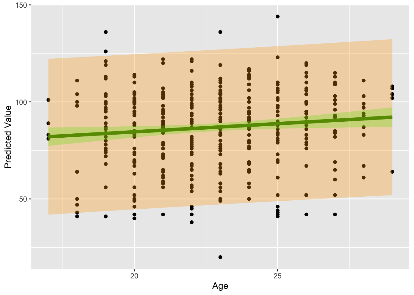
ggplot(plot_data) +
  geom_point(aes(dat.age, dat.score)) +
  geom_line(aes(dat.age,est), col = "darkgreen", lwd=2) +
  geom_ribbon(aes(x=dat.age, ymin =lwr, ymax = upr ), fill = "green", alpha = 0.3) +
  geom_ribbon(aes(x=dat.age, ymin =lwr_pred, ymax = uppr_pred ), fill = "orange", alpha = 0.3) +
  labs(x = "Age", y = "Predicted Value")

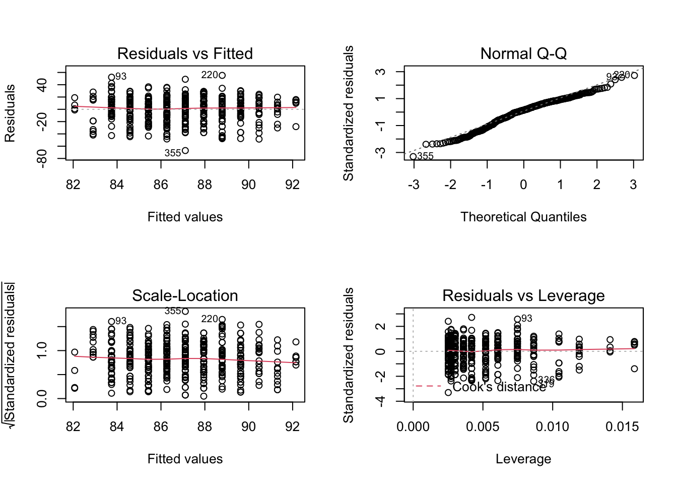
Model Diagnostics

Residual vs. Fitted

• ${\widehat{ϵ}}_i$ should be independent of ${\hat{y}}_i$, i.e., no patterns.

• Linearity: Red line should be flat, ie banded around 0.

• Constant variance (homoscedasticity).

Normal Q-Q Plot

• Standardized residual ${\widehat{ϵ}}_i/(\hat{\sigma }\sqrt{1-h_{ii}})$ should be a standard normal.

• We expect the points to follow a straight line, Check non-normality, particularly skewed tails.

Scale-Location

• Similar to residual vs fitted, but use standardized residual. Diagnose heteroscedasticity (eg red line increasing).

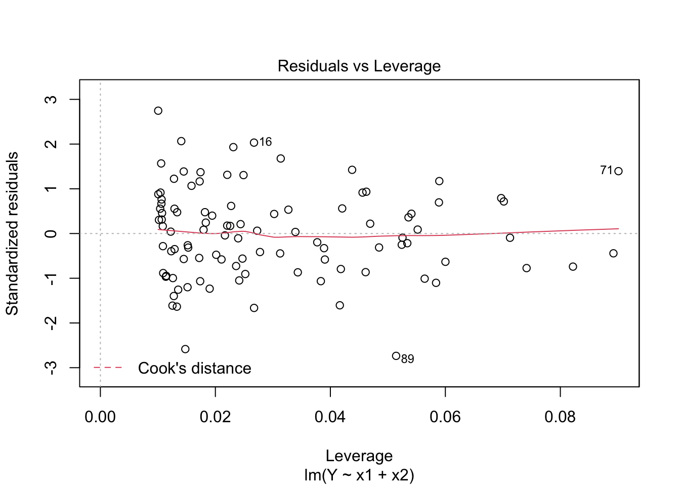
Residual vs Leverage

• Leverage $h_{ii}$ is how far away $x_i$ is from other $x_j$ where $h_{ii}=\frac{\partial {\hat{y}}_i}{\partial y_i}$.
• Cook’s Distance: measures how much model changes when remove $ith$ point; >1 is problematic.

par(mfrow=c(2,2))
plot(fit)

Hypothesis Testing

• (Intercept): $H_0:{\beta }_0=0$ when $age=0$. In other words test scores are equal to zero for a mother at $age=0$ versus $H_a:{\beta }_0\ne 0$.

• Age: $H_0:{\beta }_1=0$ In words, the slope of age is equal to zero or there is no linear effect. $H_a:{\beta }_1\ne 0$ if there is a significant linear effect.

summary(fit)

Call:
lm(formula = score ~ age, data = dat)

Residuals:
    Min      1Q  Median      3Q     Max 
-67.109 -11.798   2.971  14.860  55.210 

Coefficients:
            Estimate Std. Error t value Pr(>|t|)    
(Intercept)  67.7827     8.6880   7.802 5.42e-14 ***
age           0.8403     0.3786   2.219    0.027 *  
---
Signif. codes:  0 '***' 0.001 '**' 0.01 '*' 0.05 '.' 0.1 ' ' 1

Residual standard error: 20.34 on 398 degrees of freedom
Multiple R-squared:  0.01223,   Adjusted R-squared:  0.009743 
F-statistic: 4.926 on 1 and 398 DF,  p-value: 0.02702

Tip

In class exercise:

What conclusions can we make about the intercept and the impact of age?

Summary II

What is the model?	In multiple linear regression, we regress a vector of outcomes $Y$ values on multiple vector of predictor values $X=(X_1,X_2,...,X_p)$ with: $Y=X\beta +ϵ$ $\beta$ is a $(p+1)\times 1$ *vector of regression coefficients: the intercept* ${\beta }_0$ , and (2) the covariate coefficients $\beta =({\beta }_1,{\beta }_2,...,{\beta }_p)$.
Model Assumptions	$E(ϵ)$ is i.i.d normally distributed $N(0,{\sigma }^2)$. $Var(ϵ)={\sigma }^2$ global variance $y$ is a linear function of $x$ $y\perp ϵ$ orthogonality $=$ independence
Maximum Likelihood	$\hat{\beta }=(X^{\prime }X{)}^{-1}{X}^{\prime }y$ is the best (smallest variance) linear unbiased estimator of the true $\beta$ and is equal to ${\beta }_{GLS}$ under normality. $E(\hat{\beta })=\beta$ and $cov(\hat{\beta })={\sigma }^2(X^{\prime }X{)}^{-1}$ ${\hat{\sigma }}_{MLE}^2=\frac{1}{n}(Y-X\hat{\beta }{)}^T(Y-X\hat{\beta })$ is biased $s^2=\frac{1}{n-p}(Y-X\hat{\beta }{)}^T(Y-X\hat{\beta })$ is an unbiased estimator
Interpretation	${\beta }_0$ the global value of $E(Y)$ when $X=0$ ${\beta }_1$ the global value of the change of $Y$ for every one unit change of $X$ ${\sigma }^2$ captures the total variance across all observations but is a biased estimator
Prediction	The predicted value is given by ${\tilde{y}}_i=\hat{\beta }{X}_i+\widehat{e_i}$. The uncertainty around the predicted value is equal to ${\tilde{y}}_i\pm 1.96{\tilde{\sigma }}^2$. ${\tilde{\sigma }}^2$ is the sum of the data variance ${\widehat{sigma}}^2{x}_i^T(X^{T}X{)}^{-1}{x}_i$ and the global variance $\widehat{{\sigma }^2}$, i.e., ${\tilde{\sigma }}^2\ge {\hat{\sigma }}^2$
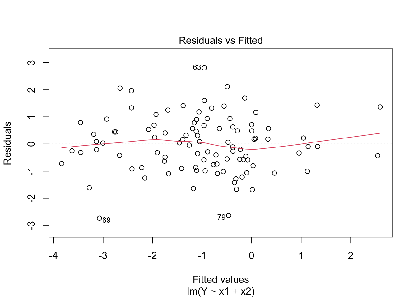
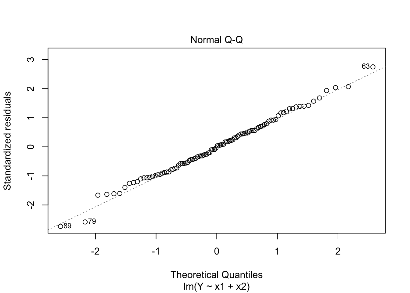
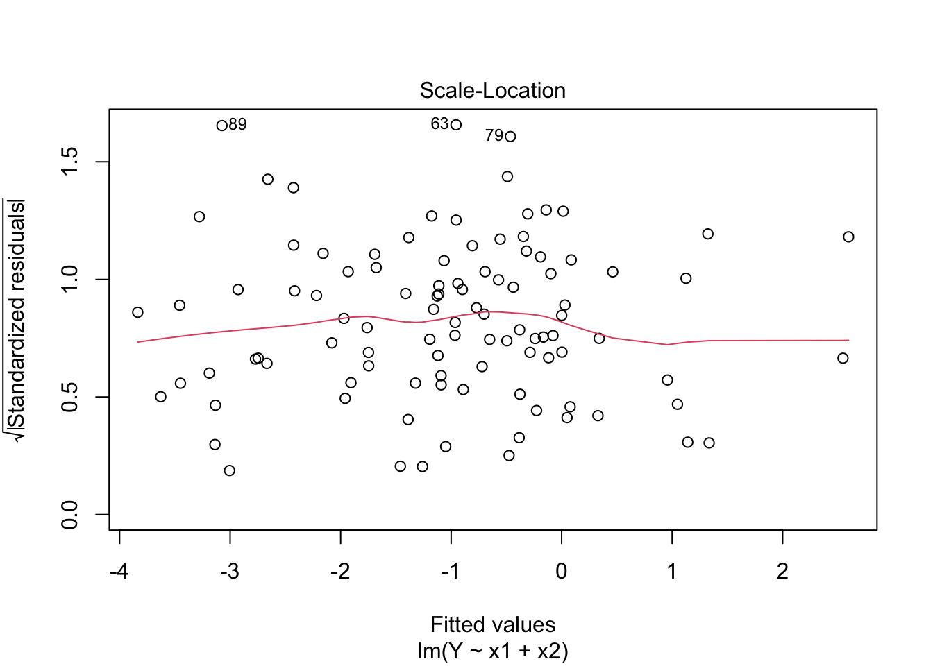
Diagnostics	Linearity: Residuals vs Fitted should be banded around 0 with constant variance, i.e., no patterns. Normality: Normal QQ Plot should follow the straight line with slightly skewed tails. Constant variance: Standardized residuals should show flat line Residual vs Leverage: Shows impact of outlier values, Cook’s distance >1 is problematic.
Hypothesis Testing	$H_0:\beta =0$ is the null hypothesis of no effect. $H_A:\beta \ne 0$ is the alternative hypothesis of a significant effect not equal to zero.

BREAKOUT SESSION 1

1. Let $H=X(X^{\prime }X{)}^{-1}{X}^{\prime }$ and let $\hat{Y}=HY$. Then $H\hat{Y}=?$
2. Show the derivation for $cov(\hat{\beta })$.
3. What is the unbiased estimator of ${\sigma }^2$?
4. The unbiased estimator for ${\sigma }^2$ contains a parameter $p$. What does $p$ represent?
5. Below code is given to simulate data from a “true” model. Run the code to get simulated quantities of covariates $X$ and outcomes $Y$.
6. What is the “true” intercept in the below simulation?
7. What is the “true” covariate coefficient value in the below simulation?
8. Fit the linear model. Find the estimates of the ${\beta }^{\prime }s$ and global variance ${\sigma }^2$.
9. Interpret the findings of the model in terms of null versus alternative hypotheses.
10. Create diagnostic plots and determine if model assumptions have been met.

set.seed(1232)
beta0 = 0.1
beta1 = 0.5
beta2 = -0.2

x1 <- rnorm(n=100, 0, 2)
x2 <- rnorm(n=100, 5, 5)
error <- rnorm(n=100, 0, 1)

X = cbind(1, x1, x2)
Beta = c(beta0, beta1, beta2)
Y = X %*% Beta + error

fit <- lm(Y~ x1+x2)
summary(fit)

Call:
lm(formula = Y ~ x1 + x2)

Residuals:
     Min       1Q   Median       3Q      Max 
-2.73778 -0.73060 -0.00343  0.64077  2.80824 

Coefficients:
            Estimate Std. Error t value Pr(>|t|)    
(Intercept) -0.12451    0.14929  -0.834    0.406    
x1           0.50463    0.05346   9.439 2.18e-15 ***
x2          -0.16957    0.02229  -7.607 1.82e-11 ***
---
Signif. codes:  0 '***' 0.001 '**' 0.01 '*' 0.05 '.' 0.1 ' ' 1

Residual standard error: 1.028 on 97 degrees of freedom
Multiple R-squared:  0.6167,    Adjusted R-squared:  0.6088 
F-statistic: 78.04 on 2 and 97 DF,  p-value: < 2.2e-16

plot(fit)

Confounding

We found that older mothers had children on average with higher test scores.

However, higher maternal education was associated with higher age as shown below.

ggplot(dat) +
  geom_boxplot(aes(as.factor(edu),age)) +
  labs(x = "Mother Education", y= "Age at Delivery")

• How do we estimate the age association with outcome accounting for the effect (confounding) of education?

Confounding

• Causes spurious correlation.

• Referred to as “omitted variable bias”

• We want to control/account for confounding associations!

• How do we account for confounding?

• Include confounders in the regression equation $\to$ MULTIPLE LINEAR REGRESSION: $y\sim x+z$

• Assumptions of linear regression plus omitted variable assumption:

  • Residuals are independent AND normal.

  • Global variance (homoscedasticity).

  • Linearity of all included covariates.

  • All variables that are not included in the model have coefficient equal to ero (omitted variable bias = 0).

Categorical Variables

• First we examine the effects of education on scores.

• $edu$ is coded as 1,2,3,4. We do NOT want to code this as continuous!!

Approach 1: an indicator (dummy) for each group.

$$X_{1i}=1_{[ed{u}_i=1]},X_{2i}=1_{[ed{u}_2=1]},X_{3i}=1_{[ed{u}_i=3]},X_{4i}=1_{[ed{u}_i=4]}$$

If we have $ed{u}_i=[1,1,2,2,3,3,4,4]$, the design matrix is

$$X\beta =\left(\begin{array}{cccc}1& 0& 0& 0\\ 1& 0& 0& 0\\ 0& 1& 0& 0\\ 0& 1& 0& 0\\ 0& 0& 1& 0\\ 0& 0& 1& 0\\ 0& 0& 0& 1\\ 0& 0& 0& 1\end{array}\right)\cdot \left(\begin{array}{c}{\beta }_1\\ {\beta }_2\\ {\beta }_3\\ {\beta }_4\end{array}\right)$$

• Note we remove the intercept. If we try to include an intercept, there is linear dependency between columns and there is no unique solution.

E1 = as.numeric(dat$edu ==1)
E2 = as.numeric(dat$edu ==2)
E3 = as.numeric(dat$edu ==3)
E4 = as.numeric(dat$edu ==4)

E1[1:6]

[1] 0 1 0 1 0 1

fit = lm(dat$score ~ E1 + E2 + E3 + E4  -1) #use -1 to remove the intercept

summary(fit)

Call:
lm(formula = dat$score ~ E1 + E2 + E3 + E4 - 1)

Residuals:
   Min     1Q Median     3Q    Max 
-58.45 -12.70   1.61  15.23  57.55 

Coefficients:
   Estimate Std. Error t value Pr(>|t|)    
E1   78.447      2.159   36.33   <2e-16 ***
E2   88.703      1.367   64.88   <2e-16 ***
E3   87.789      2.284   38.44   <2e-16 ***
E4   97.333      3.831   25.41   <2e-16 ***
---
Signif. codes:  0 '***' 0.001 '**' 0.01 '*' 0.05 '.' 0.1 ' ' 1

Residual standard error: 19.91 on 396 degrees of freedom
Multiple R-squared:  0.9508,    Adjusted R-squared:  0.9503 
F-statistic:  1913 on 4 and 396 DF,  p-value: < 2.2e-16

• What does each element of $\beta$ vector mean?
  • ${\hat{\beta }}_1$ is equivalent to taking the average of scores for kids with mother’s $edu=1$. So each $\hat{\beta }$ is equivalent to calculating the mean IQ for each education group.

In class exercise

What is the estimated difference in average score between mothers without high school and mothers with college and above?

Approach 2: Intercept plus three indicators for groups 2,3, and 4.

$X_{1i}=1,X_{2i}=1_{[ed{u}_2=1]},X_{3i}=1_{[ed{u}_i=3]},X_{4i}=1_{[ed{u}_i=4]}$

fit = lm(dat$score ~ factor(dat$edu))
summary(fit)

Call:
lm(formula = dat$score ~ factor(dat$edu))

Residuals:
   Min     1Q Median     3Q    Max 
-58.45 -12.70   1.61  15.23  57.55 

Coefficients:
                 Estimate Std. Error t value Pr(>|t|)    
(Intercept)        78.447      2.159  36.330  < 2e-16 ***
factor(dat$edu)2   10.256      2.556   4.013 7.18e-05 ***
factor(dat$edu)3    9.342      3.143   2.973  0.00313 ** 
factor(dat$edu)4   18.886      4.398   4.294 2.21e-05 ***
---
Signif. codes:  0 '***' 0.001 '**' 0.01 '*' 0.05 '.' 0.1 ' ' 1

Residual standard error: 19.91 on 396 degrees of freedom
Multiple R-squared:  0.05856,   Adjusted R-squared:  0.05142 
F-statistic:  8.21 on 3 and 396 DF,  p-value: 2.59e-05

• $\hat{\beta }$ represents the difference in average score with respect to the $edu=1$ group., i.e., 10.256 is the average difference between no high school group and high school group.

Adjusting for Confounding:

• Consider the above model: $y_i={\beta }_0+{\beta }_1{E}_{2i}+{\beta }_2{E}_{3i}+{\beta }_3{E}_{4i}+{\beta }_{4}ag{e}_i+{ϵ}_i$.

• Each education group has their own coefficient.

• The slope of maternal age is constant across education groups (parallel lines).

• ${\beta }_4$ is the association between score and age, accounting for different averages in score in different education groups.

fit = lm(score ~ factor(edu)  + age, data = dat)
summary(fit)

Call:
lm(formula = score ~ factor(edu) + age, data = dat)

Residuals:
    Min      1Q  Median      3Q     Max 
-58.853 -12.112   1.779  14.687  58.298 

Coefficients:
             Estimate Std. Error t value Pr(>|t|)    
(Intercept)   72.2360     8.8700   8.144 5.07e-15 ***
factor(edu)2   9.9365     2.5953   3.829 0.000150 ***
factor(edu)3   8.8416     3.2203   2.746 0.006316 ** 
factor(edu)4  17.6809     4.7065   3.757 0.000198 ***
age            0.2877     0.3985   0.722 0.470736    
---
Signif. codes:  0 '***' 0.001 '**' 0.01 '*' 0.05 '.' 0.1 ' ' 1

Residual standard error: 19.92 on 395 degrees of freedom
Multiple R-squared:  0.0598,    Adjusted R-squared:  0.05028 
F-statistic:  6.28 on 4 and 395 DF,  p-value: 6.59e-05

• Age effect is no longer statistically significant after accounting for mother’s education level.
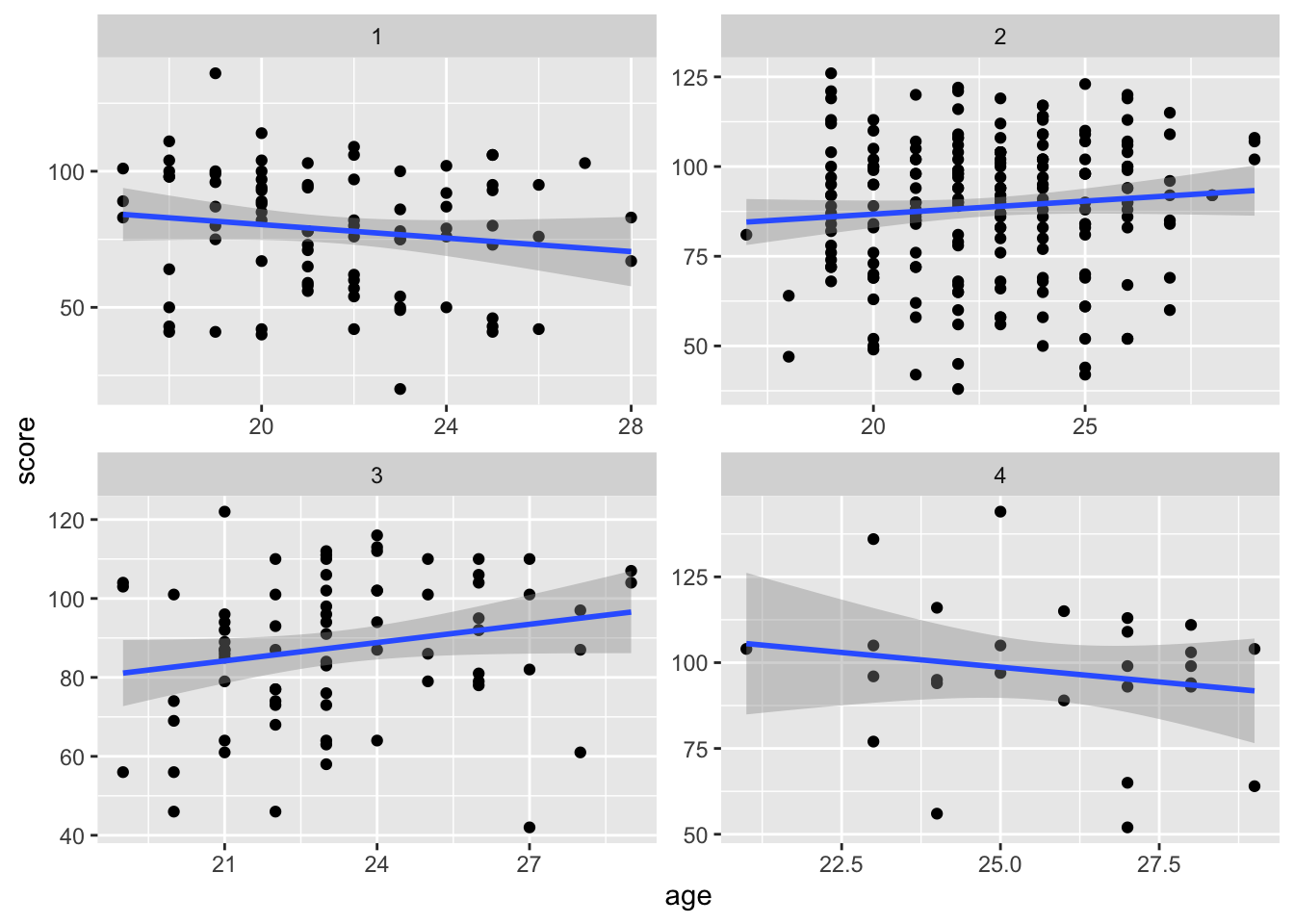
• This model assumes an identical effect of age across ALL education groups.
• Is this assumption realistic?

Variance Inflation Factors

• One must always be on the lookout for issues with multicollinearity!

• The general issues is that when two variables are highly correlated, it is hard to disentangle their effects.

• Mathematically, the standard errors are inflated. Suppose we have a design matrix $\mathbf{X}=[x_1,...,x_p]$ and we want to calculate the variance inflation factor (VIF). We regress $x_1$ against $x_2,...,x_p$.

• Let $R_1^2$ be the associated R-squared for $x_1$. Then $VI{F}_1=\frac{1}{1-R_1^2}$.

• It can be shown that $Var({\hat{\beta }}_j)=VI{F}_j\cdot \frac{{\sigma }^2}{(n-1)s_{x_j}^2}$.

• Different rules of thumb $VIFs>5$ are cause for concern.

library(car)

Loading required package: carData

vif(fit)

               GVIF Df GVIF^(1/(2*Df))
factor(edu) 1.15514  3        1.024328
age         1.15514  1        1.074774

# Is this bigger than 5. These look pretty good
temp = vif(fit)
temp[,3]^2

factor(edu)         age 
   1.049248    1.155140 

Interaction Effects: Effect Modification

• We can relax the assumption of identical age effect by inluding interaction terms.
• Again the reference group is $edu=1$ or $E_{1i}$.

$$\begin{array}{rl}{y}_i& ={\beta }_0+{\beta }_1{E}_{2i}+{\beta }_2{E}_{3i}+{\beta }_3{E}_{4i}+{\beta }_{4}ag{e}_i+\\ & {\beta }_5{E}_{2i}ag{e}_i+{\beta }_6{E}_{3i}ag{e}_i+{\beta }_7{E}_{4i}ag{e}_i+{ϵ}_i\end{array}$$

• For each edu group: We account for modified effects by examining whether ${\beta }_5,{\beta }_6$, and ${\beta }_7$ are zero.

$$y_i=\{\begin{array}{ll}{\beta }_0={\beta }_{4}ag{e}_i& \text{ if edu =1}\\ {\beta }_0+{\beta }_1+({\beta }_4+{\beta }_5)ag{e}_i& \text{ if edu =2}\\ {\beta }_0+{\beta }_2+({\beta }_4+{\beta }_6)ag{e}_i& \text{ if edu =3}\\ {\beta }_0+{\beta }_3+({\beta }_4+{\beta }_7)ag{e}_i& \text{ if edu =4}\end{array}$$

fit = lm(score ~ factor(edu) * age, data = dat)
summary(fit)

Call:
lm(formula = score ~ factor(edu) * age, data = dat)

Residuals:
   Min     1Q Median     3Q    Max 
-56.70 -11.80   2.07  14.58  54.34 

Coefficients:
                 Estimate Std. Error t value Pr(>|t|)    
(Intercept)      105.2202    17.6127   5.974  5.2e-09 ***
factor(edu)2     -33.0929    21.5732  -1.534   0.1258    
factor(edu)3     -53.4970    27.9460  -1.914   0.0563 .  
factor(edu)4      36.4537    49.5065   0.736   0.4620    
age               -1.2402     0.8097  -1.532   0.1264    
factor(edu)2:age   1.9704     0.9764   2.018   0.0443 *  
factor(edu)3:age   2.7862     1.2293   2.266   0.0240 *  
factor(edu)4:age  -0.4799     1.9635  -0.244   0.8070    
---
Signif. codes:  0 '***' 0.001 '**' 0.01 '*' 0.05 '.' 0.1 ' ' 1

Residual standard error: 19.81 on 392 degrees of freedom
Multiple R-squared:  0.07705,   Adjusted R-squared:  0.06057 
F-statistic: 4.675 on 7 and 392 DF,  p-value: 4.756e-05

vif(fit)

                        GVIF Df GVIF^(1/(2*Df))
factor(edu)     9.093097e+05  3        9.842800
age             4.821946e+00  1        2.195893
factor(edu):age 1.039839e+06  3       10.065322

• Note how the variance is inflated

• This is common with interaction variables since by construction there is dependence between an interaction variable and the main effects.

• In general, it means we need larger sample sizes to examine interactions.

• It is important to visualize the data and model results.

• We see the lines are not parallel and the intercept differs across groups.

library(ggplot2)
ggplot(dat, aes(age, score)) +
  geom_point() +
  geom_smooth(method = "lm") +
  facet_wrap(~ edu, ncol = 2, scales = "free")

`geom_smooth()` using formula = 'y ~ x'

F-test of interaction

To test whether the interaction was significant, look at whether the inclusion of the interaction significantly “improved” model fit.

• $H_0$: The interaction between education and age does not improve model fit.
• $H_A$: The interaction improves model fit.

Suppose we want to choose between these two models, i.e., Full model vs. Reduced model. We use the F-statistic:

F-statistic to perform model comparison

The F statistic is a ratio of two chi-square distributions to test whether the full model gives additional information, e.g., does ${\beta }_5={\beta }_6={\beta }_7=0$?

$$F=\frac{y^{\prime }(H_{full}-H_{reduced})y/p-1}{y^{\prime }(I-H_{full})y/n-p}=\frac{{\chi }_{p-1-k}^2/p-1-k}{X_{n-p}^2/n-p}\ge F_{\alpha ,k,n-k-1}$$

fit_inter = lm(score ~ factor(edu) * age, data = dat) #Full Model
fit_nointer = lm(score~ factor(edu) + age, data = dat) #Reduced Model
anova(fit_nointer, fit_inter)

Analysis of Variance Table

Model 1: score ~ factor(edu) + age
Model 2: score ~ factor(edu) * age
  Res.Df    RSS Df Sum of Sq      F  Pr(>F)  
1    395 156733                              
2    392 153857  3    2876.5 2.4429 0.06376 .
---
Signif. codes:  0 '***' 0.001 '**' 0.01 '*' 0.05 '.' 0.1 ' ' 1

• Overall, there is only limited statistical evidence of an interaction!
• Let’s take a closer look at the individual slopes.
• We wish to estimate the slope of $ag{e}_i$ among $Ed{u}_i=3$.

In class exercise

What is the point estimate and variance of the slope among $ed{u}_i=3$?

fit = lm(score ~ factor(edu) * age, data = dat)
Est = coef(fit)[5] + coef(fit)[7]
vcov = vcov(fit) #Gives the covariance matrix
vcov

                 (Intercept) factor(edu)2 factor(edu)3 factor(edu)4        age
(Intercept)         310.2054   -310.20544   -310.20544   -310.20544 -14.155298
factor(edu)2       -310.2054    465.40208    310.20544    310.20544  14.155298
factor(edu)3       -310.2054    310.20544    780.97662    310.20544  14.155298
factor(edu)4       -310.2054    310.20544    310.20544   2450.89473  14.155298
age                 -14.1553     14.15530     14.15530     14.15530   0.655695
factor(edu)2:age     14.1553    -20.91116    -14.15530    -14.15530  -0.655695
factor(edu)3:age     14.1553    -14.15530    -34.11363    -14.15530  -0.655695
factor(edu)4:age     14.1553    -14.15530    -14.15530    -96.63535  -0.655695
                 factor(edu)2:age factor(edu)3:age factor(edu)4:age
(Intercept)            14.1552976        14.155298        14.155298
factor(edu)2          -20.9111574       -14.155298       -14.155298
factor(edu)3          -14.1552976       -34.113627       -14.155298
factor(edu)4          -14.1552976       -14.155298       -96.635354
age                    -0.6556950        -0.655695        -0.655695
factor(edu)2:age        0.9533347         0.655695         0.655695
factor(edu)3:age        0.6556950         1.511213         0.655695
factor(edu)4:age        0.6556950         0.655695         3.855352

SE = sqrt(vcov(fit)[5,5] + vcov(fit)[7,7] + 2 * vcov(fit)[5,7])
Est

     age 
1.545989 

SE

[1] 0.9249421

• So 95% CI for the point estimate is: $$1.54\pm 1.96\times 0.92=(-0.27,3.36)$$ and thus is not statistically different from 0 at $\alpha =0.05$

Summary III

What is the model?	In multiple linear regression, we regress a vector of outcomes $Y$ values on multiple vector of predictor values $X=(X_1,X_2,...,X_p)$ with: $Y=X\beta +ϵ$ $\beta$ is a $(p+1)\times 1$ *vector of regression coefficients: the intercept* ${\beta }_0$ , and (2) the covariate coefficients $\beta =({\beta }_1,{\beta }_2,...,{\beta }_p)$. | Confounding variables results in spurious correlations because of associations with predictors and outcomes. Referred to as omitted variable bias. We ACCOUNT FOR confounders by including them in the multiple regression, i.e, $y\sim X+C$
Model Assumptions	Errors are i.i.d normal Linearity Global variance (homoscedasticity) All variables NOT included in the model have a coefficient of zero.
Effect Modification	Dummy variables: Indicators vectors of group assignment. We model the intercept plus $p-1$ indicators, using one group as a reference to avoid multicollinearity. Interaction effects $y\sim X+I+X\cdot I$ result in different intercepts and slopes across groups.
Interpretation	${\beta }_k$ is the association between $y$ and $x$ accounting for different averages in $y$ in difference groups. Without interaction, the model assumes a constant slope across groups. With interaction, the coeff for interaction $({\beta }_k+{\beta }_j)x_i$ captures the effect of the interaction between group assignment and $x$.
Diagnositcs	*Variance Inflation (VIF) occurs when there is multicollinearity. $Var({\hat{\beta }}_j)=VI{F}_j\cdot \frac{{\sigma }^2}{(n-1)s_{x_j}^2}$ where $VI{F}_j=\frac{1}{1-R_j^2}$ $VIF>5$ is problematic.
Hypothesis Testing	F-test of interaction tests whether the interaction was significant. Test for model comparison between full and simple model. $H_0=$ interaction does not improve model fit. $H_A=$ interaction does improve model fit.