Module 3: Generalized Linear Models

Loading required package: Matrix

Attaching package: 'lmerTest'

The following object is masked from 'package:lme4':

    lmer

The following object is masked from 'package:stats':

    step

Reading

• Chapter 3, Wood S. Generalized Additive Models, 2017. Has a nice self-contained introduction to generalized linear models.
• Gelman & Hill. Data Analysis using Regression and Multilevel/Hierarchical Models.2006.
• https://en.wikipedia.org/wiki/Generalized_linear_model

Basic Concepts

• Models for non-normal data

• Link functions

• Logistic regression: Binary data

• Probit regression: Binary data

• Poisson regression: Count data

Consider the following multiple linear regression model: For \(i=1, ..., n\).

\[ y_i = \beta_0 + \sum_{k=1}^K \beta_k x_{ik} + \epsilon_i \qquad e_i \overset{iid}{\sim} N(0, \sigma^2) \]

This is equivalent to \(y_i \sim N(\beta_0 + \sum_{k=1}^K \beta_k x_{ik} , \sigma^2)\) where \(x_{ik}\) is the kth linear predictor for observation \(i\).

Reminder of the assumptions of the above model:

• The \(\beta's\) are fixed unknown constants.
• \(y\) is a linear function of the covariates.
• The expectation of the errors \(e's\) is zero.
• Only \(\epsilon's\) are random.

Therefore, \(y_i\) follows a normal distribution and the \(E(y_i|x_i) = \beta_0 + \sum_{k=1}^K \beta_k x_{ik}\). The linear regression part is used to model the mean function of \(y_i\). The assumptions do not hold for other kinds of data, i.e, binary, count data, etc.

Generalized Linear Regression Model

A generalized linear model (GLM) extends the linear regression to other distributions, where the response variable is generated from a distribution in the exponential family.

A GLM involves three ingredients:

1. A probability distribution in the Exponential Family.

2. A linear model \(x_i'\beta\).

3. A link function \(g()\) and its inverse \(g^{-1}()\) is the link that relates the linear model to the expectation, i.e., transforms the mean function to meet the linear model assumptions.

   \[ \begin{align*} E(y_i|x_i) & = \mu_i = g^{-1} (x_i\beta)\\ Var(y_i|x_i) & = V(\mu_i) =V(g^{-1}(x_i\beta)) \end{align*} \]

4. Note: Unlike OLS, the basic form of the GLM does not involve a noise variance (no \(\sigma^2\)).

Exponential Family

The basic form for an exponential family density is

\[ f_{\theta} (y) = exp[\{y\theta - b(\theta)\} / a(\phi) + c(y, \phi )] \]

where \(a, b, c\) are known functions, and \(\phi\) is a known scale parameter. The ONLY parameter is \(\theta\).

In the GLM, \(\theta\) will be a function of \(x_i\beta\).

Examples of distributions in the exponential family include: normal with known variance (link = identity), Bernoulli (link = logit or probit), binomial (link = logit or log), gamma, exponential (link = negative inverse), and others.

• Lets derive a general class for the exponential function.

Let’s take a binary outcome where \(p_i\) is the probability of success. For \(i=1,...,n\) assume \[ y_i \sim Bernoulli (p_i) \]

where \(p_i \in (0,1)\) and the Bernoulli function has the following characteristics:

\[ \begin{align*} E(y_i) & = p_i\\ Var(y_i) & =V(p_i) = p_i (1- p_i)\\ f(y_i|p_i) & = p_i ^{y_i} (1-p_i)^{1-y_i} \end{align*} \]

We know that \(\mu_i = p_i = P(Y_i=1)\). So we wish to model a link function \(g()\) the enforces a linear relationship between the unscaled expectation \(\mu_i\) and the expectation \(\beta_0 + \sum_{k=1}^K \beta_k x_{ik}\), i.e, we wish to model

\[ g(\mu_i) = \beta_0 + \sum_{k=1}^K \beta_k x_{ik} \] The two most commonly used link functions are the logistic function , and the probit function.

The link function should have some desirable properties:

1. \(g()\) should have a range \((-\infty, \infty)\) so that \(\beta's\) and \(X's\) can have any value.
2. \(g()\) should have a domain that corresponds to all possible values of \(\mu_i\), i.e., \((0,1)\) for the binomial distribution.
3. \(g()\) should be one-to-one \(\mu_i = g^{-1}(\beta_0 + \sum_k \beta_k X_{ik})\).
4. \(g()\) should be strictly increasing, i.e., \(g(p_i) \rightarrow \infty\) when \(p_i \rightarrow 1\).

Logistic Regression

For a logistic regression, we use the logit link function defined as:

\[ g(p_i) = log\left(\frac{p_i}{1-p_i}\right) = \beta_0 + \sum_k \beta_k X_{ik}, \qquad (0,1) \rightarrow (-\infty, \infty) \]

Meaning \(log(p_i/1-p_i) \rightarrow -\infty\) when \(p_i \rightarrow 0\) and \(log(p_i/1-p_i)\rightarrow \infty\) when \(p_i \rightarrow 1\).

In general the logistic function is defined as :

\[ p_i = \frac{e^{g(\mu_i)}}{1 + e^{g(\mu_i)}} = \frac{1}{1+ e^{-g(\mu_i)}}, \qquad (-\infty, \infty) \rightarrow (0,1) \]

• The \(\beta's\) are estimated using the iterative re-weighted MLE method.

• There is no \(\epsilon_i\)!!! Meaning the variance is not defined by a normally distributed noise term.

• \(g(p_i)\) is interpreted as the log_odds of probability of success.

Interpretation:

When \(X_i=0\), \(log(\frac{p_i}{1-p_i}) = \beta_0\) which is interpreted as the baseline or reference log-odds of probability.

\(\beta_1\) is interpreted as the CHANGE in log-odds per one unit change in \(X_i\). Conversely, \(e^{\beta_1}\) is defines the odds-ratio.

\[ log(\frac{p_i}{1-p_i}) = \beta_0 + \beta_1 x_i, \text{ versus } log(\frac{p^*_i}{1-p^*_i}) = \beta_0 + \beta_1 (x_i + 1) \]

then

\[ log\left(\frac{p^*_i /1-p^*_i}{p_i /1-p_i}\right) = \beta_1 \]

In the multiple logistic regression, \(\beta_k\) is the log odds ratio associated with covariate \(k\) while controlling for other covariates.

The Odds Ratio:

Odds Ratio interpretation is helpful for indicator variables. Let \(x_i=1\) in exposed group and \(x_i=0\) in unexposed group. Then:

\[ e^{\beta_1} = \frac{\{\frac{p(y_i=1|x_i=1}{p(y_i=0|x_i=1}\}}{\frac{p(y_i=1|x_i=0}{p(y_i=0|x_i=-}\}} = \frac{\text{odds(Exposed)}}{\text{odds(Unexposed)}} \]

• OR>1 means a positive association

• OR<1 means a negative association

• OR=1 means no difference between exposure groups.

It is really important to understand that the change in log-odds per one unit change in \(X_i\) is not constant, i.e, that change in log-odds depends on the value of \(X_i\).

#The Logit Function
p.i <- seq(0, 1, by = 0.001)
g_p.i <- log(p.i/(1-p.i))
plot(p.i, g_p.i, col = "red", xlab ="p", ylab = "Logit Function")

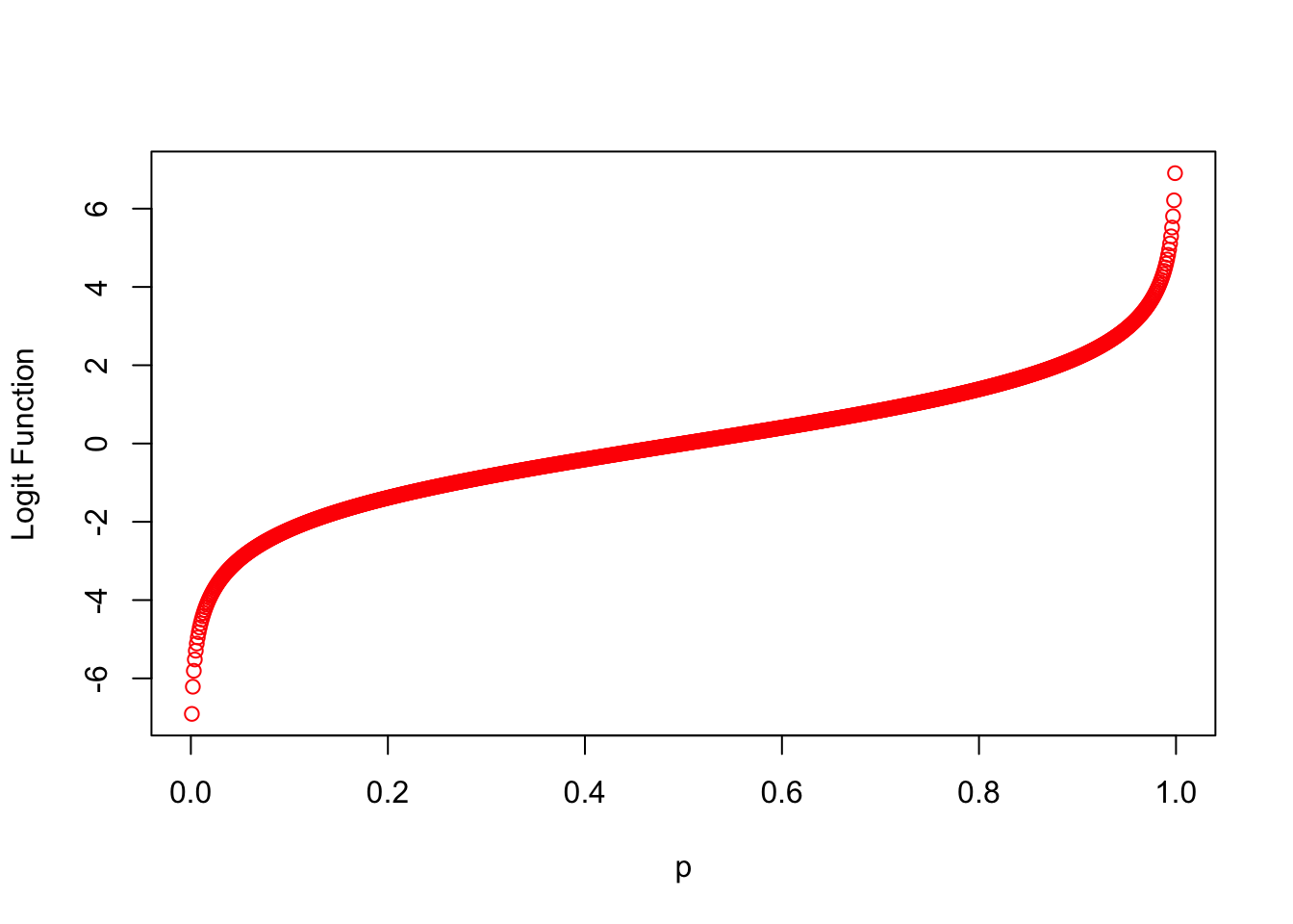
#The Logistic Function
p_i <- exp(g_p.i)/(1+exp(g_p.i))
plot(g_p.i, p_i, col = "blue", xlab = "x", ylab = "Logistic Function")

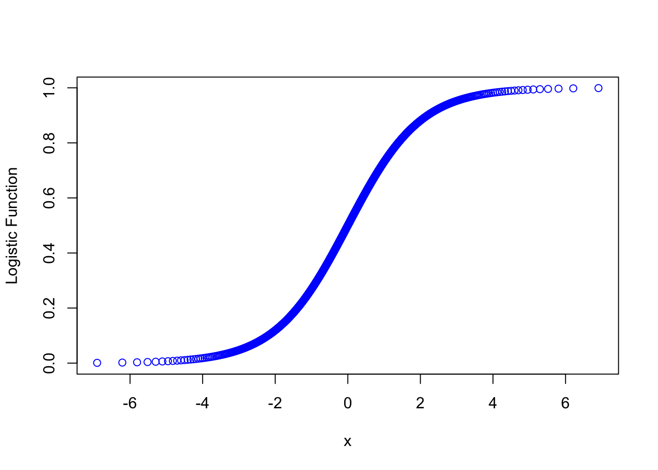
What are the effects of changing the baseline odds?

\[ \begin{align} logit(p_i)& = \beta_0 + x_i\\ \mu_i = P(Y_i =1) &= \frac{e^{\beta_0 + x_i}}{1 + e^{\beta_0 + x_i}} \end{align} \]

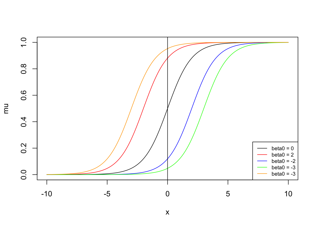
Note: The shape is maintained, and the baseline (intercept) probability changes.

What are the effects of the change in slope?

\[ \begin{align} logit(p_i)& = \beta_1 x_i\\ \mu_i = P(Y_i =1) = \frac{e^{\beta_1 x_i}}{1 + e^{\beta_1 x_ii}} \end{align} \]

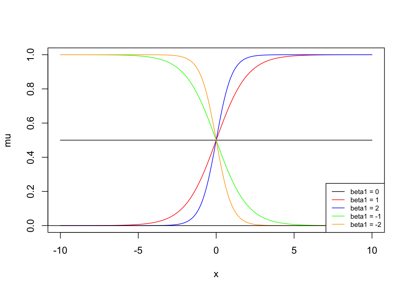
Note how the steepness changes with difference in slopes. Also note how the direction changes depending on the effect changes.

Fitting a logistic regression in R

Motivating Example

The dataset: a cohort of live births from Georgia born in the year 2001 \(N = (77,340)\).

Variables:

• ptb: indicator for whether a baby from pregnancy \(i\) was born preterm (<37 weeks).

• age: the mother’s age at delivery (centered at age 25).

• male: indicator of the baby’s sex (1=male, 0=female)

• tobacco: indicator for mother’s tobacco use during pregnancy (1= yes, 0 = no).

Tobacco is treated as the exposure variables. Mothers age is a covariate.

Fitting the GLM model in R is very similar to fitting a linear regression model. We need to specify the distribution as binomialand the link function as logit.

### The GLM Function

load("/Users/emilypeterson/Library/CloudStorage/OneDrive-EmoryUniversity/BIOS 526/BIOS526_Book/data/PTB.Rdata")

fit <- glm(formula = ptb ~ age + male + tobacco, 
    family = binomial(link = "logit"),
    data = dat)

summary(fit)

Call:
glm(formula = ptb ~ age + male + tobacco, family = binomial(link = "logit"), 
    data = dat)

Deviance Residuals: 
    Min       1Q   Median       3Q      Max  
-0.5160  -0.4236  -0.4103  -0.4088   2.2500  

Coefficients:
              Estimate Std. Error z value Pr(>|z|)    
(Intercept) -2.4212664  0.0631355 -38.350  < 2e-16 ***
age         -0.0006295  0.0021596  -0.291  0.77068    
maleM        0.0723659  0.0258672   2.798  0.00515 ** 
tobacco      0.4096495  0.0534627   7.662 1.83e-14 ***
---
Signif. codes:  0 '***' 0.001 '**' 0.01 '*' 0.05 '.' 0.1 ' ' 1

(Dispersion parameter for binomial family taken to be 1)

    Null deviance: 44908  on 77339  degrees of freedom
Residual deviance: 44846  on 77336  degrees of freedom
AIC: 44854

Number of Fisher Scoring iterations: 5

• Preterm delivery was significantly associated with male babies (p-value = 0.005) when controlling for age and mother’s smoking status. The odds ratio of a preterm birth for a male baby versus a female baby was 1.07 (95% CI: 1.02, 1.13).

• \(OR = e^{0.0723} = 1.07\) with 95% CI = (1.02, 1.13).

  • How we get CIs: \(e^{(0.0723 \pm 1.96 * 0.0258)}\).

    NOTE: TRANSFORM THE INTERVALS. DO NOT TRANSFORM THE STANDARD ERRORS (this requires the delta method).

• Preterm delivery was significantly associated with whether the mother smoked during pregnancy (p<0.001) when controlling for age and the baby’s sex.

• \(OR = e^{0.409} = 1.51 (1.36, 1.67)\).

• The baseline proportion (female babies born to mother of age 25 who didn’t smoke) of preterm delivery was

  \[ \frac{e^{-2.42}}{1 + e^{-2.42}} = 0.08. \]

• We didn’t find an effect of mother’s age.

Likelihood Ratio Test

• How can we test whether which model is better?

• The likelihood for a binary logistic regression is given by:

\[ L(\beta; \mathbf{y}, \mathbf{X}) = \prod_{i=1}^{n} \pi_i^{y_i} (1-\pi_i)^{1-y_i} \]

• This yields a log-likelihood of:

\[ \begin{align*} l(\beta) &= \sum_{i=1}^n [y_i log(\pi_i) + (1-y_i) log(1-\pi_i)\\ &= \sum_{i=1}^n [y_i \mathbf{X}_i \beta - log(1+ exp(\mathbf{X}_i \beta))] \end{align*} \]

• Maximizing the LL has no closed form solution, so a technique used to obtain MLEs \(\hat{\beta}\) is iteratively reweighted least squares (no covered here).

The likelihood ratio test (LRT) is used to test the null hypothesis that any subset of the \(\beta's\) is equal to 0. The number of \(\beta's\) in the full model is \(k+1\), while the number of \(\beta's\) in the reduced model is \(r+1\). (Remember the reduced model is the model that results when the \(\beta's\) in the null hypothesis are set to 0). Thus, the number of \(\beta's\) being tested in the null hypothesis is \((k+1) - (r+1) = k-r\).

• LRT requires the simpler (null) model is nested within the larger model.

• The Likelihood Ratio Test is given by: \[ LR= \frac{max_{H_0}L(\beta)}{max_{H_A}L(\beta)} \]

• This gives the ratio of the likelihood of the null model evaluated at the MLEs to the likelihood of the full model evaluated at the MLEs.

• In the normal case, this is the analogous to the F-test described in Chapter 1.

• The likelihood ratio test statistic is given by:

  \[ \lambda_{LR} = -2[l(\hat{\beta}_{reduced}) - l(\hat{\beta}_{full})] \]

• The difference follows a Chi-square distribution, i.e.,

  \[ \lambda_{LR} > \chi^2_{\nu, 1-\alpha} \]

where \(\nu\) denotes the different in number of parameters, i.e., \(k-r\) = degrees of freedom.

library(car)

Loading required package: carData

Anova(fit)

Analysis of Deviance Table (Type II tests)

Response: ptb
        LR Chisq Df Pr(>Chisq)    
age        0.085  1   0.770669    
male       7.834  1   0.005126 ** 
tobacco   53.648  1  2.399e-13 ***
---
Signif. codes:  0 '***' 0.001 '**' 0.01 '*' 0.05 '.' 0.1 ' ' 1

Wald Test

The Wald Test is the test of significance for individual regression coefficients in logistic regression. Wald test under regularity conditions and assuming asympotitc results,

\[ \begin{align} \hat{\beta} &\sim N(\beta, I(\beta)^{-1})\\ I(\beta) &= E\left\{\left(\frac{\partial l}{\partial \beta}\right)\left(\frac{\partial l}{\partial \beta}\right)'\right\}\\ &= -E\frac{\partial^2 l}{\partial \beta \partial \beta'} \end{align} \]

• \(I(\beta)\) is called the Fisher information matrix (see Wood p.106).

• We can write \(\hat{\beta} \sim N(\beta, (\mathbf{X'} \mathbf{W} \mathbf{X})^{-1} \phi)\) where \(\mathbf{W}\) contains the “Fisher weights” and \(\phi=1\) in the usual (not overdispersed) GLM.

• In \(R\) the default \(summary(glmmodel)\) is a Wald-type test.

• For maximum likelihood estimates, the ratio

\[ Z = \frac{\hat{\beta}_i}{s.e.(\hat{\beta}_i)} \]

can be used to test \(H_0: \beta_i =0\). The standard normal curve is used to determine the \(p-value\) of the test.

–> –> –>

–>

Population versus Conditional Interpretations

• The GLM is estimating the marginal model (integrating out the random effect, commonly we assume they are zero).

\[ g(E[y_{ij}]) = \beta X_{ij} \]

This is known as the population-averaged effect or marginal effect.

• The GLMM is estimating the slopes conditioned on the random effects:

\[ g(E[y_{ij}|\theta_i]) = \beta X_{ij} + \theta_i \] These slopes are estimated controlling for subject effects, which are called conditional effects.

• The two approaches are estimating different slopes!.

• Note: the GLM likelihood assumes independence, resulting in incorrect SE.

• We are modeling transformations of the expectations:

\[ E(y_{ij}|\theta_i) = g^{-1}(\beta_0 + \theta_i + \sum_{k=1}^p \beta x_{ijk}) \] - For Gaussian (GLM), \(g()\) is the identity function, so slopes in the marginal model have same interpretation as the conditional model:

\[ E(y_{ij}) = E[E(y_{ij}|\theta_i)] = E[\beta_0 + \theta_i + \beta'X_{ij}] = \beta_0 + \beta'X_{ij} \]

• For GLMMs, we have

\[ E[y_{ij}] = E[E(y_{ij} |\theta_i)] = E[g^{-1} (\beta_0 + \theta_i + \beta'X_{ij})] \ne g^{-1}( E(\beta_0 + \theta_i + \beta'X_{ij})) \]

Poisson Regression

• The Poisson model is used for count data, that is; where each data point \(y_i\) can equal 0,1,2,….

\[ y_i \sim Poisson(\theta_i) = \frac{e^{-\theta_i}\theta_i^{y_i}}{y_i !} \]

• As with linear and logistic regression, the variation in \(y\) can be explained with linear predictors \(X\).

\[ \theta_i = exp(X_i \beta) \]

• Here the link is the log(). log() has domain \((0, \infty)\) and range \((-\infty, \infty)\) and is strictly increasing.

Differences between the Binomial and Poisson models

The Poisson model is similar to the binomial model for county data but is applied in slightly different situations.

• If each data point \(y_i\) can be interpreted as the number of “successes” out of \(n_i\) trials then it is standard to use the binomial/logistic model.

• If each data point \(y_i\) does not have a natural limit- it is not based on a number of independent trials- then it is standard to use the Poisson/log repression model.

Poisson Regression Interpretation

• Consider a simple Poisson regression model with only one covariate:

\[ \begin{align*} y_i &\overset{ind}{\sim} Pois(\lambda_i)\\ log(\lambda_i) & = \beta_0 + \beta_1 x_i \end{align*} \]

• When \(x_i=0\) then \(log(\lambda_i) = \beta_0\). So \(e^{\beta_0} = \lambda_i\) is the baseline expected count and \(\lambda_i\) is the rate.

• Now consider a unit change in \(x\).

  \[ \begin{align*} log(\lambda_i) & =\beta_0 + \beta_1 x_i\\ log(\lambda_i^*) & = \beta_0 + \beta_1 (x_i + 1)\\ \beta_1 & = log(\lambda^*_i) - log(\lambda_i)\\ \end{align*} \]

• \(e^{\beta_1}\) is the relative change in count per unit change in x. Also called the relative rate. Also called the incidence ratio.

• Covariate impacts are multiplicative rather than additive (apples to log models in general) on the count scale.

Motivating Example: Cancer Incidence in Ohio

Let \(s\) index one of the 88 counties in Ohio, \(t\) index year, and \(k\) index a population sex-race stratum.

Variables:

• \(death_{stk}\): stratified lung cancer death counts for population \(k\) in county \(s\) during year \(t\).

• \(sex_k\): 1=female, 0=male.

• \(race_k\): 1= white, 0 = nonwhite.

• \(year_t\): 1,2,…,9 for year 1980 to 1988.

• \(pop_{stk}\): at risk population size.

Questions: - What were the associations between lung cancer death counts and sex/race.

• Estimate the between-county variation in lung cancer risks.

• County level estimation is within the field of small-area estimation.

cancer <- readRDS(paste0("data/ohio_cancer.RDS"))
head(cancer)

  county sex race year death   pop
1      1   1    1    1     6  8912
2      1   1    1    2     5  9139
3      1   1    1    3     8  9455
4      1   1    1    4     5  9876
5      1   1    1    5     8 10281
6      1   1    1    6     5 10876

Consider a random-intercept Poisson model where we treat all stratified death counts within the same county as a group.

\[ \begin{align*} death_{stk} &\sim Poisson(\theta_{stk})\\ log(E(death_{stk}|\theta_s)) & = \beta_0 + \theta_s + \beta_1 I_{sex_k=Female} + \beta_2 I_{race_k = white} \\ & + \beta_3 I_{sex_k = female, race_k = white} \end{align*} \]

Interpretation:

• \(\beta_0=\) log expected lung cancer death count at baseline (non-white males in 1979) for the average county.

• \(\theta_s=\) county-specific deviations in baseline log expected lung cancer by county \(s\).

• \(e^{\beta_1}=\) ratio of lung cancer deaths for non-white female to non-white male in a model accounting for county-specific random intercepts, year, and interaction between sex and race.

• \(e^{\beta_2}=\) ratio of lung cancer deaths for white males compared to non-white males.

• \(e^{\beta_3}=\) relative rate modification in deaths for white females, e.g., \(e^{\beta_1 + \beta_2 + \beta_3}\) is the rate ratio in white females to non-white males.

fit = lme4::glmer(death ~ factor(sex)*factor(race) +  (1|county),
            family = poisson, data =cancer)
summary(fit)

Generalized linear mixed model fit by maximum likelihood (Laplace
  Approximation) [glmerMod]
 Family: poisson  ( log )
Formula: death ~ factor(sex) * factor(race) + (1 | county)
   Data: cancer

     AIC      BIC   logLik deviance df.resid 
 39383.0  39417.6 -19686.5  39373.0     7387 

Scaled residuals: 
    Min      1Q  Median      3Q     Max 
-7.4474 -1.0870 -0.6149  0.4008 14.8303 

Random effects:
 Groups Name        Variance Std.Dev.
 county (Intercept) 1.094    1.046   
Number of obs: 7392, groups:  county, 88

Fixed effects:
                            Estimate Std. Error  z value Pr(>|z|)    
(Intercept)                 2.839322   0.111674   25.425  < 2e-16 ***
factor(sex)2               -1.014711   0.007458 -136.061  < 2e-16 ***
factor(race)2              -2.064819   0.011466 -180.087  < 2e-16 ***
factor(sex)2:factor(race)2 -0.165960   0.023499   -7.062 1.64e-12 ***
---
Signif. codes:  0 '***' 0.001 '**' 0.01 '*' 0.05 '.' 0.1 ' ' 1

Correlation of Fixed Effects:
            (Intr) fctr(s)2 fctr(r)2
factor(sx)2 -0.018                  
factor(rc)2 -0.012  0.173           
fctr()2:()2  0.006 -0.317   -0.488  

Poisson Regression

An alternative parametization of Poisson regression models an incidence rate and not an expected count. Consider the model where we incorporate the population-at-risk, i.e., the total population or a subset of the population, etc.

\[ \begin{align*} y_{stk}& \sim Poisson (\theta_{stk})\\ \theta_{stk} & = N_{stk} * exp(\mu_{stk})\\ log(\theta_{stk}) & = log(N_{stk})+ \mu_{stk}\\ \mu_{stk} & = \beta_0 + \theta_s + \beta_1 sex_k + \beta_2 race_k + \beta_3 sex_k \times race _k \\ \theta_s & \sim N(0, \tau^2) \end{align*} \]

The log-population \(log(N_{stk})\) is referred to as the offset. In other words, \(\frac{y_{stk}}{N_{stk}} \sim Pois(exp(\mu_{stk}))\).

\(\theta_{stk}/N_{stk} = exp(\beta_0 + \theta_s + \beta_1 sex_k + \beta_2 race_k + \beta_3 sex_k \times race _k )\).

Here \(e^{\beta_0}\) is interpreted as the baseline per capita deaths, instead of the expected counts (for a nonwhite male in year 1979 conditioning on county). It is the fraction of deaths per person, i.e., per capita death rate.

cancer$logpop = log(cancer$pop)

fit = lme4::glmer(death ~ offset(logpop) + factor(sex)*factor(race) +  (1|county),
            family = poisson,
            data = cancer)

summary(fit)

Generalized linear mixed model fit by maximum likelihood (Laplace
  Approximation) [glmerMod]
 Family: poisson  ( log )
Formula: death ~ offset(logpop) + factor(sex) * factor(race) + (1 | county)
   Data: cancer

     AIC      BIC   logLik deviance df.resid 
 31814.5  31849.0 -15902.2  31804.5     7387 

Scaled residuals: 
    Min      1Q  Median      3Q     Max 
-7.8261 -0.6352 -0.2335  0.4472  9.8153 

Random effects:
 Groups Name        Variance Std.Dev.
 county (Intercept) 0.03991  0.1998  
Number of obs: 7392, groups:  county, 88

Fixed effects:
                            Estimate Std. Error  z value Pr(>|z|)    
(Intercept)                -7.367370   0.022071 -333.808  < 2e-16 ***
factor(sex)2               -1.077799   0.007458 -144.510  < 2e-16 ***
factor(race)2               0.034907   0.011735    2.974  0.00293 ** 
factor(sex)2:factor(race)2 -0.219521   0.023503   -9.340  < 2e-16 ***
---
Signif. codes:  0 '***' 0.001 '**' 0.01 '*' 0.05 '.' 0.1 ' ' 1

Correlation of Fixed Effects:
            (Intr) fctr(s)2 fctr(r)2
factor(sx)2 -0.089                  
factor(rc)2 -0.030  0.171           
fctr()2:()2  0.029 -0.317   -0.476  

In class exercise

We are going to implement a more realistic Poisson regression model to explore the associations of sex and race on cancer incidence in Ohio.

1. Read in the Ohio cancer data from Canvas.

2. Create exploratory plots of the associations/relationships between

   1. Sex and Number of deaths.
   2. Race and Number of deaths.
   3. Cancer Incidence by County.
   4. Write up a paragraph that explains the findings from the exploratory analysis, and how this motivates model assumptions.

3. Run a Poisson regression in R using the following model:

\[ \begin{align*} y_{stk}& \sim Poisson (\theta_{stk})\\ \theta_{stk} & = N_{stk} * exp(\mu_{stk})\\ log(\theta_{stk}) & = log(N_{stk})+ \mu_{stk}\\ \mu_{stk} & = (\beta_{0cr}) + \beta_{1} sex_k + \beta_3 sex_k \times race _k \\ \beta_{0cr} & = \beta_0 + \theta_{cr}, \quad \theta_{cr} \sim N(0, \tau^2) \end{align*} \]

Hint: the intercept can be broken down into two rand effects in the \(glmer()\) function, (1|county) + (1|race)

4. What does this model described above implement, are is the assumptions of the model valid based on your exploratory findings?

5. What were the findings from the R output?

Overdispersion of the Poisson Assumption

• In Poisson, the assumption \(E(y_i) = V(y_i)\) is often violated!

• One can add an additional overdispersion parameter also called a scale parameter.

• One can adjust the parameter variance by this scale parameter. This is called the quais-poisson model.

  \[ \hat{\mathbf{\beta}} \sim N(0, I(\mathbf{\beta})^{-1} \phi) \]

• Fitting a quasi-poisson in GLM

glm_quasi = glm(death ~ offset(logpop) + factor(sex)*factor(race) +  (1|county),
            family = "quasipoisson",
            data = cancer)

summary(glm_quasi)

Call:
glm(formula = death ~ offset(logpop) + factor(sex) * factor(race) + 
    (1 | county), family = "quasipoisson", data = cancer)

Deviance Residuals: 
    Min       1Q   Median       3Q      Max  
-7.1212  -0.9661  -0.3920   0.2381  10.6459  

Coefficients: (1 not defined because of singularities)
                            Estimate Std. Error   t value Pr(>|t|)    
(Intercept)                -7.280397   0.005707 -1275.600  < 2e-16 ***
factor(sex)2               -1.074482   0.011065   -97.106  < 2e-16 ***
factor(race)2               0.117448   0.017011     6.904 5.47e-12 ***
1 | countyTRUE                    NA         NA        NA       NA    
factor(sex)2:factor(race)2 -0.218442   0.034865    -6.265 3.93e-10 ***
---
Signif. codes:  0 '***' 0.001 '**' 0.01 '*' 0.05 '.' 0.1 ' ' 1

(Dispersion parameter for quasipoisson family taken to be 2.200393)

    Null deviance: 43628  on 7391  degrees of freedom
Residual deviance: 15976  on 7388  degrees of freedom
AIC: NA

Number of Fisher Scoring iterations: 5

Hierarchical Models

Concepts

• Hierarchical linear models: three level random intercept model for Gaussain data ( a type of lmm).

• Hierarchical generalized linear models (a type of glmm).

• Hierarchical structure and covariance structures.

Reading

• School data example adapted from Gelman and Hill.

• Guatemalan data example: Rodriguez B and Goldman N (2001). Improved estimation procedures for multilevel models with binary response: a case study. Journal of Royal Statistical Society Series A 339-355.

Motivating Example

Level 1 (year within child): finest level: values vary with \(k\).

• \(math_{ijk}\): math scores (outcome)

• \(year_{ijk}\): primary school year centered at 3.5.

• \(retained_{ijk}\): indicator for child \(ij\) repeating the grade in year \(k\).

Level 2 (child within school): values vary with \(j\) (constant over \(k\)).

• \(child_{ij}\): child Id.

• \(female_{ij}\): indicator for child \(i\) in school \(j\) being female.

• \(black_{ij}\): indicator for child \(i\) in school \(j\) being African American

• \(hispanic_{ij}\) : indicator for child \(i\) in school \(j\) being Hispanic.

Level 3 (school): values vary with \(i\): highest (most granular) level (constant over \(j\) and \(k\))

• \(school_i\): school ID.

• \(size_i\): number of students in school \(i\).

• \(lowinc_i\): percent of students from low-income families in school \(i\).

Three-Level Normal Random Intercept Model

Level 1: relating math scored to occasion (year) specific covariates:

\[ math_{ijk} = \beta_{0,ij} + \beta_1 year_{ijk} + \beta_2 retained_{ijk} + \epsilon_{ijk} \]

Level 2: relating child-specific random intercepts to child. characteristics

\[ \beta_{0,ij} = \alpha_{0,i} + \alpha_1 female_{ij} + \alpha_2 black_{ij} + \alpha_3 hispanic_{ij} + \phi_{ij} \]

Level 3: relating school-specific random intercepts to school characteristics.

\[ \alpha_{0,i} = \gamma_0 + \gamma_1 size_i + \gamma_2 lowinc_i + \eta_i \]

\[ \begin{align*} \epsilon_{ijk}& \overset{iid}{\sim} N(0, \sigma^2)\\ \phi_{ij} & \overset{iid}{\sim} N(0, \tau^2)\\ \eta_i& \overset{iid}{\sim} N(0, \nu^2) \end{align*} \]

Interpretation:

• Level 1:

  • A child’s score in year \(k\) is a linear function of \(year_{ijk}\) and \(retained_{ijk}\)

  • \(\beta_{0,ij}\) is the child-specific random intercept. Note that the coefficient has a subscript \(ij\) as it cannot be influenced by variables that change between school years.

  • Between-child variation is accounted for by \(\beta_{0,ij}\).

  • After removing the child-specific intercept ( and year and retained effects), residual variation in math scores follow \(N(0, \sigma^2)\).

• Level 2:

  • This second-level regression models explains variation in \(\beta_{0,ij}\).

  • We assume \(\beta_{0,ij}\) is a linear function of child specific covariates \(female_{ij}, black_{ij}\) and \(hispanic_{ij}\).

  • \(\alpha_{0,i}\) is a school-level random intercept. It captures correlation in \(\beta_{0,ij}\) for children from the same school.

  • Variation in child-specific \(\beta_{0,ij}\) not explained by child-level covariates and the school-level intercepts follow \(N(0, \tau^2)\).

• Level 3:

  • Levels 3 explains variation in school-specific intercepts \(\alpha_{0,i}\) using school-level covariates \(sie_i\) and \(lowinc_i\).

  • We assume \(\alpha_{0,i}\) is normal with variance \(\nu^2\).

  • \(\gamma_0\) is the overall baseline mean math score across 60 schools. Here the baseline is 0% low-income students and zero students.

  • \(\gamma_1\) can be interpreted as: increase in school-average math score per unit increase in \(size_i\).

Reparametrization of the multi-level model: The multilevel model can be combined to give:

\[ \begin{align*} math_{ijk} &= \gamma_0 + \gamma_1 size_i + \gamma_2 lowinc_i + \eta_i \\ & \alpha_1 female_{ij} + \alpha_2 black_{ij} + \alpha_3 hispanic_{ij} + \phi_{ij}\\ & \beta_1 year_{ijk} + \beta_2 retained_{ijk} + \epsilon_{ijk}\\ \epsilon_{ijk} & \overset{iid}{\sim}N(0, \sigma^2)\\ \phi_{ij} & \overset{iid}{\sim}N(0, \tau^2)\\ \eta_{i} & \overset{iid}{\sim}N(0, \nu^2) \end{align*} \]

• Because \(size_i\) and \(lowinc_i\) are the same values for all scores taken in a particular school \(\gamma_1\) and \(\gamma_2\) change \(math_{ijk}\) on the school-level.

• Every measurement and every child in school \(i\) has the same \(\gamma_1 size_i + \gamma_2 lowinc_i + \eta_i\).

• \(\gamma_0\) is the overall mean math score at baseline:

  • \(size_i = 0\) and \(lowinc_i=0\)

  • male, non-Black, non-Hispanic

  • grade year at 3.5 not retained.

Within-child correlation = correlation between different scores within the same child (must be within the same school).

• What is \(Var(math_{ijk})\)?

• What is \(Cov(math_{ijk}, math_{ijk'})\)?

• What is \(Cor(math_{ijk}, math_{ijk'})\)?

Intra-school correlation: Correlation between different scores within the same chool (different child)

• What is \(Cov(math_{ijk}, math_{ij'k'})\)?

• What is \(Cor(math_{ijk}, math_{ij'k'})\)?

Note that within-child scores are more similar than within school scores.

Note that in a nested-structure, we don;t have data from the same child but different schools.

Hierarchical Specification of the multi-level model:

\[ \begin{align*} math_{ijk} & \sim N(\beta_{0,ij} + \beta_1 year_{ijk} + \beta_2 retained_{ijk}, \sigma^2 )\\ \beta_{0,ij} & \sim N( \alpha_{0,i} + \alpha_1 female_{ij} + \alpha_2 black_{ij} + \alpha_3 hispanic_{ij}, \tau^2 )\\ \alpha_{0,i} & \sim N( \gamma_0 + \gamma_1 size_i + \gamma_2 lowinc_i, \nu^2) \end{align*} \]

Hierarchical Model Fitting in R

dat <- read.csv(paste0(getwd(), "/data/achievement.csv"))
dim(dat)

[1] 7230   10

dat[1:6,]

  year   math retained female black hispanic size lowinc school child
1  0.5  1.146        0      0     0        1  380   40.3   2020   244
2  1.5  1.134        0      0     0        1  380   40.3   2020   244
3  2.5  2.300        0      0     0        1  380   40.3   2020   244
4 -1.5 -1.303        0      0     0        0  380   40.3   2020   248
5 -0.5  0.439        0      0     0        0  380   40.3   2020   248
6  0.5  2.430        0      0     0        0  380   40.3   2020   248

We specify the multi-level model with two random intercept components. (Here child ID is unique, so the below code is equivalent to (1|school) + (1|school:child), see R code)

dat <- read.csv(paste0(getwd(), "/data/achievement.csv"))
fit <- lmer(math~ year + retained + female + black + hispanic + size + lowinc + (1|school) + (1|child), data = dat)
summary(fit)

Linear mixed model fit by REML. t-tests use Satterthwaite's method [
lmerModLmerTest]
Formula: math ~ year + retained + female + black + hispanic + size + lowinc +  
    (1 | school) + (1 | child)
   Data: dat

REML criterion at convergence: 16706.4

Scaled residuals: 
    Min      1Q  Median      3Q     Max 
-3.8439 -0.5837 -0.0267  0.5587  6.1702 

Random effects:
 Groups   Name        Variance Std.Dev.
 child    (Intercept) 0.6637   0.8147  
 school   (Intercept) 0.0875   0.2958  
 Residual             0.3445   0.5870  
Number of obs: 7230, groups:  child, 1721; school, 60

Fixed effects:
              Estimate Std. Error         df t value Pr(>|t|)    
(Intercept)  2.398e-01  1.524e-01  6.406e+01   1.573  0.12064    
year         7.483e-01  5.396e-03  5.744e+03 138.685  < 2e-16 ***
retained     1.481e-01  3.535e-02  5.802e+03   4.190 2.83e-05 ***
female      -9.038e-05  4.223e-02  1.668e+03  -0.002  0.99829    
black       -5.182e-01  8.060e-02  1.154e+03  -6.429 1.88e-10 ***
hispanic    -2.899e-01  8.910e-02  1.642e+03  -3.254  0.00116 ** 
size        -1.028e-04  1.485e-04  5.719e+01  -0.692  0.49167    
lowinc      -8.002e-03  1.818e-03  6.900e+01  -4.401 3.84e-05 ***
---
Signif. codes:  0 '***' 0.001 '**' 0.01 '*' 0.05 '.' 0.1 ' ' 1

Correlation of Fixed Effects:
         (Intr) year   retand female black  hispnc size  
year     -0.012                                          
retained -0.009  0.086                                   
female   -0.141 -0.005  0.017                            
black    -0.108 -0.006 -0.013 -0.006                     
hispanic -0.071 -0.010 -0.006  0.018  0.556              
size     -0.454 -0.009  0.008 -0.019  0.025 -0.079       
lowinc   -0.622  0.009 -0.009  0.015 -0.326 -0.188 -0.221

Note that the random effects of child and school are assumed to be independent.

• Within-child correlation \(= \frac{0.66 + 0.087}{0.66 + 0.087 + 0.34} = 0.69\).
• Within-school correlation \(=\frac{0.087}{0.66 + 0.087 + 0.34} = 0.08\).

Note on nesting A child is nested within school because for a given child, school does not vary. Therefore, we can’t look at the interaction between child and school!. We can only look at interactions for crossed factors. There are many possible interactions here.

The higher number of interactions, the finer the level (the smaller the sample). So to keep things simple, we will ignore them here.

Interpretation:

• Across schools, children, and school years, the average math score is 0.2398 for baseline measurement (year = 3.5, retained = 0, female = 0, Black = 0, Hispanic = 0, size = 0, lowinc = 0 , ave school and ave child). Intercept is not meaningful here.

• Lower child-specific average math scores were associated with African American and Hispanic students.

• Lower school-specific average math scores were associated with schools with higher proportion of low-income students.

• Math scores increased as a child progressed in grade.

• Math scores higher for grades that a child repeated (retained).

Study Limitations

• \(lowinc\) is the proportion of students at a school that are lower income (level 3 covariate).

• We cannot estimate whether a student from a disadvantaged background (low income, single family household, parents’ education, others) has lower scores.

• In particular, race and ethnicity are correlated with other factors impacting on individual’s achievement scores.

• The lower scores reflect products of systemic racism and shortcomings of the education system.

• Results of this data set could be used to help prioritize education funds or policy.

Comparison with 2-Level Models

• Our 3-level model decomposes the total residual variation into three components:

  • Level 3: Between school variation \(\nu^2\).

  • Level 2: Between child variation \(\tau^2\).

  • Level 1: Between grade variation (within a child) \(\sigma^2\).

  We can consider models that only include random intercepts for schools or for children.

  Assume no between-child variation

  # fit2 <- lmer (math ~ year + retained + female + black + hispanic + size + lowinc + (1|school) , data = dat)

  Assume no between-school variation

  # fit3 <- lmer (math ~ year + retained + female + black + hispanic + size + lowinc + (1|child) , data = dat)

Selecting Random Effects

1. Fit the above “simplified models (fits 2 and 3) in R.
2. Compare all three model fits using \(anova(fit2, fit)\) and \(anova(fit3, fit)\).
3. Based on AIC, which is the preferred model choice?

Note: Likelihood Ratio Tests can be inaccurate due to issues of testing a null hypothesis on the boundary of the parameter space (generally, p-values too big). I suggest using a model that seems reasonable.

Hierarchical GLMMs

Motivating Example: Guatemalan Vaccination Data

• Cross-sectional study of families’ decision to immunize their children.

• Surveyed 1,595 mothers in 161 communities in Guatemala in 1987.

• Collected children immunization status born in the previous 5 years.

• Scientific question: (1) whether a campaign in 1986 increased immunization rate, (2) were children at least 2-years old at time of interview more likely to be immunized?

• Outcome data will \(y_{ijk}\) has three levels:

  • Level 3: Community \(i\)

  • Level 2: Family \(j\)

  • Level 1: Child \(k\)

  The data are nested: child nested in family nested in community.

Nesting Structure

• Level 1: (\(kth\) child within mother)

  • \(immun_{ijk}\): indicator for the child being immunized (outcome).

  • \(kid2p_{ijk}\): indicator for the child being at least 2-years old at interview = 1 if true, 0 if false.

• Level 2: ( \(jth\) family within community)

  • \(mom_{ij}\): mother’s (family) ID

  • \(momEduPri_{ij}\) : indicator for mother having primary education.

  • \(momEduSec_{ij}\): indicator for mother having secondary education.

  • \(husEduPri_{ij}\): indicator for husband having primary education.

  • \(husEduSec_{ij}\): indicator for husband having secondary education.

• Level 3: ( \(ith\) community)

  • \(cluster_i\): community ID

  • \(rural_i\): indicator for rural community

  • \(pcInd81_i\): percent population that was indigenous in 1981.

dat <- read.csv(paste0(getwd(), "/data/guatemalan.csv"))
dim(dat)

[1] 2159   10

head(dat)

  mom cluster immun kid2p momEdPri momEdSec husEdPri husEdSec rural   pcInd81
1   2       1     1     1        0        1        0        1     0 0.1075042
2 185      36     0     1        1        0        1        0     0 0.0437295
3 186      36     0     1        1        0        0        1     0 0.0437295
4 187      36     0     1        1        0        1        0     0 0.0437295
5 188      36     0     1        1        0        0        0     0 0.0437295
6 188      36     1     1        1        0        0        0     0 0.0437295

length(unique(dat$mom)) #Total number of mothers

[1] 1595

length(unique(dat$cluster)) #Total number of communities

[1] 161

table(table(dat$mom)) #Number of children per mom

   1    2    3 
1063  500   32 

Three Level Logistic Random Intercept Model

\[ \begin{align*} immun_{ijk} & \sim Binomial (p_{ijk})\\ logit(p_{ijk}) & = \beta_0 + u_i + u_{ij} + \beta_1'x_{ijk} + \beta_2' x_{ij} + \beta_3' x_i\\ u_{ij} & \overset{iid}{\sim} N(0, \tau^2)\\ u_i & \overset{iid}{\sim} N(0, \nu^2) \end{align*} \]

• \(x_{ijk}=[kid2p_{ijk}]\)

• \(x_{ij} = [momEduPri_{ij}, momEduSec_{ij}, husEduPri_{ij}, husEduSec_{ij}]\)

• \(x_i = [rural_i, pcInd81_i]\)

• \(\tau^2\) = between-family variation in baseline log odds.

• \(\nu^2\)=between-community variation in baseline log odds.

• Only two normal random effects.

• We can think of \(u_i\) and \(u_{ij}\) as parameters that control for unmeasrured confounders at the community and family level. One statistician’s mean structure is another’s covariance structure.

What is \(Var(immun_{ijk} |u_i, u_{ij})\)?

Recall the model is conditioned on the random effects:

\[ \begin{align*} immun_{ijk} &\sim Binomial(E(y_{ijk}|u_i, u_{ij}])\\ logit(E[y_{ijk}|u_i, u_{ij}])& =\beta_0 + u_i + u_{ij} + \beta_1' x_{ijk} + \beta_2' x_{ij} + \beta_3' x_i\\ u_{ij} & \overset{iid}{\sim} N(0, \tau^2)\\ u_i & \overset{iid}{\sim} N(0, \nu^2) \end{align*} \]

Hierarchical GLMM Fitting in R

set.seed(123)
fit <- glmer(immun ~ kid2p + momEdPri + momEdSec + husEdPri + husEdSec + rural + pcInd81 + (1|mom) + (1|cluster), family = binomial, data = dat)

Warning in checkConv(attr(opt, "derivs"), opt$par, ctrl = control$checkConv, :
Model failed to converge with max|grad| = 0.0260502 (tol = 0.002, component 1)

summary(fit)

Generalized linear mixed model fit by maximum likelihood (Laplace
  Approximation) [glmerMod]
 Family: binomial  ( logit )
Formula: immun ~ kid2p + momEdPri + momEdSec + husEdPri + husEdSec + rural +  
    pcInd81 + (1 | mom) + (1 | cluster)
   Data: dat

     AIC      BIC   logLik deviance df.resid 
  2739.8   2796.6  -1359.9   2719.8     2149 

Scaled residuals: 
    Min      1Q  Median      3Q     Max 
-1.5854 -0.6356 -0.3569  0.6972  2.4860 

Random effects:
 Groups  Name        Variance Std.Dev.
 mom     (Intercept) 1.2357   1.1116  
 cluster (Intercept) 0.5033   0.7094  
Number of obs: 2159, groups:  mom, 1595; cluster, 161

Fixed effects:
            Estimate Std. Error z value Pr(>|z|)    
(Intercept)  -0.7610     0.2800  -2.718  0.00658 ** 
kid2p         1.2812     0.1581   8.106 5.24e-16 ***
momEdPri      0.2793     0.1470   1.900  0.05749 .  
momEdSec      0.2858     0.3248   0.880  0.37884    
husEdPri      0.3763     0.1457   2.583  0.00979 ** 
husEdSec      0.3262     0.2733   1.194  0.23257    
rural        -0.6690     0.2049  -3.266  0.00109 ** 
pcInd81      -0.9823     0.2486  -3.951 7.79e-05 ***
---
Signif. codes:  0 '***' 0.001 '**' 0.01 '*' 0.05 '.' 0.1 ' ' 1

Correlation of Fixed Effects:
         (Intr) kid2p  mmEdPr mmEdSc hsEdPr hsEdSc rural 
kid2p    -0.450                                          
momEdPri -0.343  0.106                                   
momEdSec -0.234  0.073  0.350                            
husEdPri -0.355  0.091 -0.154 -0.067                     
husEdSec -0.281  0.014 -0.172 -0.474  0.394              
rural    -0.542 -0.075 -0.003  0.109  0.052  0.197       
pcInd81  -0.438 -0.108  0.195  0.105  0.024  0.046  0.050
optimizer (Nelder_Mead) convergence code: 0 (OK)
Model failed to converge with max|grad| = 0.0260502 (tol = 0.002, component 1)

What warning is this??

Convergence issues can happen for several reasons:

• Model complexity: The model may be too complex, with too many random effects or predictors that cause instability in the estimation process.

• Insufficient data: You might not have enough data to estimate all parameters properly, especially for random effects.

• Scaling issues: Poor scaling of variables can make the optimization problem numerically unstable.

• Starting values: Sometimes, the optimizer doesn’t start close enough to a good solution.

• Use the control argument in glmer to allow more iterations or to relax convergence criteria.

fit_opt <- glmer(immun ~ kid2p + momEdPri + momEdSec + husEdPri + husEdSec + rural + pcInd81 + (1|mom) + (1|cluster), family = binomial, data = dat, control = glmerControl(optimizer = "bobyqa", optCtrl = list(maxfun = 2e5)))

summary(fit_opt)

Generalized linear mixed model fit by maximum likelihood (Laplace
  Approximation) [glmerMod]
 Family: binomial  ( logit )
Formula: immun ~ kid2p + momEdPri + momEdSec + husEdPri + husEdSec + rural +  
    pcInd81 + (1 | mom) + (1 | cluster)
   Data: dat
Control: glmerControl(optimizer = "bobyqa", optCtrl = list(maxfun = 2e+05))

     AIC      BIC   logLik deviance df.resid 
  2739.8   2796.6  -1359.9   2719.8     2149 

Scaled residuals: 
    Min      1Q  Median      3Q     Max 
-1.5874 -0.6355 -0.3568  0.6970  2.4865 

Random effects:
 Groups  Name        Variance Std.Dev.
 mom     (Intercept) 1.2373   1.1123  
 cluster (Intercept) 0.5038   0.7098  
Number of obs: 2159, groups:  mom, 1595; cluster, 161

Fixed effects:
            Estimate Std. Error z value Pr(>|z|)    
(Intercept)  -0.7624     0.2801  -2.722  0.00649 ** 
kid2p         1.2815     0.1581   8.105 5.26e-16 ***
momEdPri      0.2793     0.1470   1.899  0.05753 .  
momEdSec      0.2808     0.3248   0.864  0.38735    
husEdPri      0.3771     0.1457   2.588  0.00966 ** 
husEdSec      0.3308     0.2734   1.210  0.22628    
rural        -0.6686     0.2049  -3.263  0.00110 ** 
pcInd81      -0.9824     0.2487  -3.950 7.83e-05 ***
---
Signif. codes:  0 '***' 0.001 '**' 0.01 '*' 0.05 '.' 0.1 ' ' 1

Correlation of Fixed Effects:
         (Intr) kid2p  mmEdPr mmEdSc hsEdPr hsEdSc rural 
kid2p    -0.450                                          
momEdPri -0.343  0.106                                   
momEdSec -0.234  0.072  0.349                            
husEdPri -0.355  0.091 -0.154 -0.067                     
husEdSec -0.281  0.015 -0.172 -0.474  0.394              
rural    -0.542 -0.075 -0.003  0.109  0.052  0.196       
pcInd81  -0.438 -0.108  0.195  0.106  0.024  0.045  0.050

Heterogeneity Interpretations

Interpretation:

• Baseline = rural community with 0% below poverty, mother and husband did not have primary or secondary education, and the child was under 2 years old. Baseline prob of immunization for a typical (population average) child in a model, controlling for family and community random intercept, is

  \[ \frac{e^{-0.7624}}{1 + e^{-0.7624}} = 0.32 \]

• Between-family variation contributes more than between-community variation.

• The total variation in baseline log odds has a standard deviation of \(\sqrt{1.237 + 0.504} = 1.32\). 95% of the baseline probabilities are within:

  \[ \frac{e^{-0.7624 \pm 1.96 \times 1.32}}{1 + e^{-0.7624 \pm 1.96 \times 1.32}} = (0.03, 0.87) \]

• After controlling for within-family and within-community correlation:

  • Odds of immunization decreased in rural communities (OR: \(e^{-0.67} = 0.51\), a 49% decrease), and communities with higher percentage of indigenous population: \(1-e^{-0.98 \times 0.1} = 0.093\), a 9% decrease for 10% increase in indigenous population).

  • Higher immunization rate was associated with families where the mother (OR: \(e^{0.28} = 1.31\)) or husband (OR: \(e^{0.38} = 1.46\)) received primary education vs without primary education. No significant effects for secondary edu (smaller sample size).

  • Children born during the campaign had a higher immunization rate (OR: \(e^{1.28}=3.59\)).

Regression Coefficients

• What is the odds ratio for a child at least 2 years old (kid2p=1) vs less than 2 years old (kid2p=0) for a child from the same family and community, holding other vars constant?

  • Hint: The community and family random intercepts cancel out because we are holding them constant.

• What is the OR and 95% CI in immunization between two children from the same community and same mother with

  • child B = over 2 years old at interview, mother’s husband had primary education

  • child A = under 2 years old at interview, mother’s husband had no primary education.