Module 5 Part 1: Basis Expansion and Parametric Splines

Reading

Chapter 5- Elements of Statistical Learning (Hastie)
Chapter 5- Introduction to Statistical Learning (James et al. )

Basic Concepts

Basis Functions and knots
Piecewise Linear Splines
Piecewise Cubic Splines
Bias-Variance Tradeoff
Criteria for model prediction performance (CV, GCV, AIC).

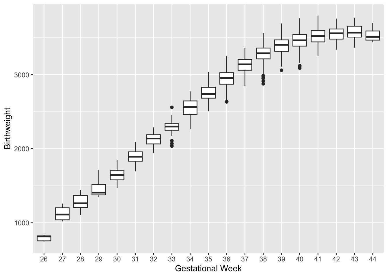
Parametric Splines

Motivating Example: Birthweight and Mothers Age

$g w$ : gestational age in weeks.
$a g e$ : maternal age at delivery
$b w$ birthweight at delivery in grams

We see a non-linear relationship between $g w$ and $b w$ of a newborn.

Let’s fit a linear regression here


Call:
lm(formula = bw ~ gw, data = dat)

Residuals:
    Min      1Q  Median      3Q     Max 
-761.50  -83.01   16.80  100.80  348.80 

Coefficients:
             Estimate Std. Error t value Pr(>|t|)    
(Intercept) -2177.513     39.351  -55.34   <2e-16 ***
gw            141.808      1.019  139.10   <2e-16 ***
---
Signif. codes:  0 '***' 0.001 '**' 0.01 '*' 0.05 '.' 0.1 ' ' 1

Residual standard error: 144.2 on 4998 degrees of freedom
Multiple R-squared:  0.7947,    Adjusted R-squared:  0.7947 
F-statistic: 1.935e+04 on 1 and 4998 DF,  p-value: < 2.2e-16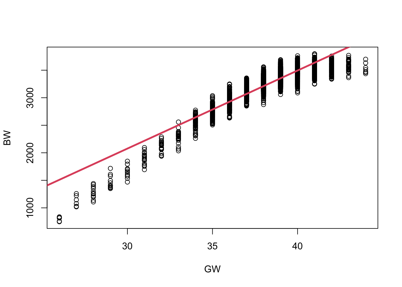

Important

Basis Expansion

Consider the regression model:

$y_{i} = g (x_{i}) + ϵ_{i}$

One approach: assume $g (x_{i})$ is a linear combination of $M$ functions of $x_{i}$ .

$g (x_{i}) = \sum_{m = 1}^{M} β_{m} b_{m} (x_{i})$

We choose and fix $b_{m} (x_{i})$ so it is known!.
We estimate the coefficients/scalars for the transformed $b_{m} (x_{i})$ .
Note! $b_{m} ()$ is simply a transformation of the original variable $x_{i}$ .
$b_{m} (x_{i})$ is called a Basis Function.
Basis functions are a core tool in the field of functional data analysis and optimizations. We model non-linear curves as piecewise functions.

What are some Bases Expansion Examples?
- Polynomial
- Indicator
- Periodic

Let’s fit a Polynomial Regression to the birthweight outcomes:

$\begin{aligned} Quadratic y_{i} & = β_{0} + β_{1} x_{i} + β_{2} x_{i}^{2} + e_{i} \\ Cubic y_{i} & = β_{0} + β_{1} x_{i} + β_{2} x_{i}^{2} + + β_{3} x_{i}^{3} + e_{i} \end{aligned}$

Note that polynomial functions often cannot model the ends very well.

Piecewise Regression

To model non-linear relationship: divide range of the covariates into some “suitable” regions. E.g. pregnancy length: preterm (<37 weeks), full-term (37-41 weeks), and post-term (>42 weeks).
Model with polynomial functions separately within each region. The interior values that define the regions (cut-points) are called knots.

Piecewise regression is equivalent to a model where the basis functions of $x_{i}$ interact with dummy variables for regions, e.g.,

$\begin{aligned} y_{i} & = β_{0} + β_{1} x_{i} + β_{2} x_{i}^{2} + β_{3} D_{1 i} \\ + β_{4} x_{i} \times D_{1 i} + β_{5} x_{i}^{2} \times D_{1 i} \\ + β_{6} D_{2 i} + β_{7} x_{i} \times D_{2 i} + β_{8} x_{i}^{2} \times D_{2 i} \end{aligned}$

where

$D_{1 i} = {\begin{cases} 1 & 37 \leq x_{i} < 42 \\ 0 & O W \end{cases}$

D_{2i} =

{\begin{cases} 1 & x_{i} \geq 42 \\ 0 & O W \end{cases}

We have two cut-points (knots) which yields three regions. We only need two dummy variables for three regions.

The positive association between pregnancy length and birth weight decreases for higher gestational weeks.
Here, linear, quadratic, and cubic result in similar trends in each regions.
Importantly! All three have discontinuities, i.e., they are not continous in the 1st and/or 2nd derivative.


Call:
lm(formula = bw ~ (gw + I(gw^2)) * (Ind1 + Ind2), data = dat)

Residuals:
    Min      1Q  Median      3Q     Max 
-403.65  -73.97    5.35   78.00  299.04 

Coefficients:
                   Estimate Std. Error t value Pr(>|t|)    
(Intercept)      -4.962e+03  8.043e+02  -6.169 7.42e-10 ***
gw                2.312e+02  5.005e+01   4.619 3.96e-06 ***
I(gw^2)          -3.160e-01  7.735e-01  -0.409    0.683    
Ind1TRUE         -2.142e+04  1.959e+03 -10.937  < 2e-16 ***
Ind2TRUE         -4.984e+04  5.279e+04  -0.944    0.345    
gw:Ind1TRUE       1.202e+03  1.045e+02  11.494  < 2e-16 ***
gw:Ind2TRUE       2.488e+03  2.470e+03   1.007    0.314    
I(gw^2):Ind1TRUE -1.685e+01  1.410e+00 -11.950  < 2e-16 ***
I(gw^2):Ind2TRUE -3.134e+01  2.889e+01  -1.085    0.278    
---
Signif. codes:  0 '***' 0.001 '**' 0.01 '*' 0.05 '.' 0.1 ' ' 1

Residual standard error: 109.6 on 4991 degrees of freedom
Multiple R-squared:  0.8816,    Adjusted R-squared:  0.8814 
F-statistic:  4646 on 8 and 4991 DF,  p-value: < 2.2e-16


Call:
lm(formula = bw ~ (gw + (gw^2)) * (Ind1 + Ind2), data = dat)

Residuals:
    Min      1Q  Median      3Q     Max 
-396.28  -74.28    4.34   78.34  321.34 

Coefficients:
             Estimate Std. Error t value Pr(>|t|)    
(Intercept) -4634.537     74.286  -62.39   <2e-16 ***
gw            210.735      2.158   97.67   <2e-16 ***
Ind1TRUE     4244.229     94.153   45.08   <2e-16 ***
Ind2TRUE     7710.241    711.475   10.84   <2e-16 ***
gw:Ind1TRUE  -114.351      2.620  -43.65   <2e-16 ***
gw:Ind2TRUE  -199.521     16.853  -11.84   <2e-16 ***
---
Signif. codes:  0 '***' 0.001 '**' 0.01 '*' 0.05 '.' 0.1 ' ' 1

Residual standard error: 111.8 on 4994 degrees of freedom
Multiple R-squared:  0.8766,    Adjusted R-squared:  0.8764 
F-statistic:  7092 on 5 and 4994 DF,  p-value: < 2.2e-16

Piecewise polynomials have limitations:
- Positive association between pregnancy length and birthweight decreases for higher gestational weeks.
- Linear, quadratic, and cubic result in similar trend in each region.
Limitations
- The regression functions do not match at knot locations.
- Requires many regression coefficients (degrees of freedom).

Linear Splines

Splines are basis functions for piecewise regressons that are connected at the interior knots.
Splines are continuous, which makes them aesthetically appealing.

A linear piecewise spline at knot locations 36.5 and 41.5 is specified as:

$y_{i} = β_{0} + β_{1} x_{i} + β_{2} (x_{i} - 36.5)_{+} + β_{3} (x_{i} - 41.5)_{+} + ϵ_{i}$

For $x_{i} < 36.5$

$y_{i} = β_{0} + β_{1} x_{i}$

For $36.5 \geq x_{i} < 41.5$

$\begin{aligned} y_{i} & = β_{0} + β_{1} x_{i} + β_{2} (x_{i} - 36.5) \\ = (β_{0} - β_{2} * 36.5) + (β_{1} + β_{2}) x_{i} \end{aligned}$

For $41.5 \geq x_{i}$

$\begin{aligned} y_{i} & = β_{0} + β_{1} x_{i} + β_{2} (x_{i} - 36.5) + β_{3} (x_{i} - 41.5) \\ = (β_{0} - β_{2} * 36.5 - β_{3} * 41.5) + (β_{1} + β_{2} + β_{3}) x_{i} \end{aligned}$

$β_{2}$ and $β_{3}$ represent changes in slope compared to the previous region.

Note here we only need 4 regression coefficients compared to 6 in the model that does not force connections at knots.

#Linear Splines
Sp1 = (dat$gw - 36.5) * as.numeric(dat$gw >= 36.5)
Sp2 = (dat$gw - 41.5) * as.numeric(dat$gw >= 41.5)
fit7 <- lm(bw ~ gw + Sp1 + Sp2, data = dat)

morepoints = seq(26, 44, .1)
newdata = data.frame(gw=morepoints, Sp1= (morepoints-36.5), Sp2=(morepoints-41.5) )
# non-zero for values greater than 36.5 and greater than 41.5 only:
newdata[ newdata <0] = 0

plot (dat$bw~dat$gw, xlab = "Gestational Week", ylab = "Birth weight")
lines (fit4$fitted[Ind1]~dat$gw[Ind1], col = 2, lwd = 3)
lines (fit4$fitted[Ind2]~dat$gw[Ind2], col = 2, lwd = 3)
lines (fit4$fitted[!Ind1 & !Ind2]~dat$gw[!Ind1 & !Ind2], col = 2, lwd = 3)

lines (predict (fit7, newdata=newdata)~morepoints, col = 4, lwd = 3)
abline (v=c(36.5, 41.5), col = "grey", lwd = 3)
legend ("topleft", legend=c("Piecewise linear", "Linear splines"), col=c(2,4), lwd=3)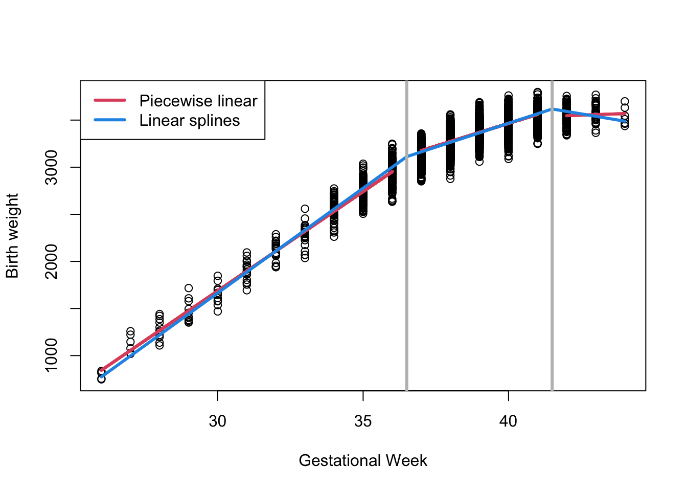

summary(fit7)


Call:
lm(formula = bw ~ gw + Sp1 + Sp2, data = dat)

Residuals:
    Min      1Q  Median      3Q     Max 
-387.65  -75.73    5.05   79.96  325.15 

Coefficients:
             Estimate Std. Error t value Pr(>|t|)    
(Intercept) -5013.768     62.747  -79.90   <2e-16 ***
gw            222.620      1.757  126.71   <2e-16 ***
Sp1          -121.427      2.549  -47.64   <2e-16 ***
Sp2          -152.948     10.492  -14.58   <2e-16 ***
---
Signif. codes:  0 '***' 0.001 '**' 0.01 '*' 0.05 '.' 0.1 ' ' 1

Residual standard error: 113 on 4996 degrees of freedom
Multiple R-squared:  0.874, Adjusted R-squared:  0.8739 
F-statistic: 1.155e+04 on 3 and 4996 DF,  p-value: < 2.2e-16

Interpretation:

223g 95%CI=(219, 226) increase in birthweight for a one week increase in gestational time prior to week 36.5.
Drops by 121 to 101.2g/week for gestation time over 36.5 weeks and less then 41.5 weeks.
After 41.5 weeks, birth weight was negatively associated with gestational week by -52g/week (95% CIs = -72, -32).

Cubic Splines

Linear splines are easily interpretable.
The resulting function $g (x_{i})$ is NOT smooth. The 1st deriv is discontinuous at the knots.
Instead we can work with piecewise cubic functions that are connected at the knots, i.e., 1st and 2nd derivs are continous (ensures continuity and smoothness):

$g (x_{i}) = β_{0} + β_{1} x_{i} + β_{2} x_{i}^{2} + β_{3} x_{i}^{3} + β_{4} (x_{i} - 36.5)_{+}^{3} + β_{5} (x_{i} - 41.5)_{+}^{3}$

Cubic splines are popular because continuous 2nd derivs, typically view as a smooth function.

#Cubic Splines
Sp1 = (dat$gw - 36.5)^3*as.numeric(dat$gw >= 36.5 )
Sp2 = (dat$gw - 41.5)^3*as.numeric(dat$gw >= 41.5)
fit8 = lm (bw~ gw+I(gw^2) + I(gw^3) + Sp1 + Sp2, data = dat)

plot(dat$gw, dat$bw, col = "black", xlab = "GW", ylab = "BW")
abline(v = 36.5)
abline(v = 41.5)
lines (predict (fit7, newdata=newdata)~morepoints, col = "red", lwd = 3)
lines(sort(dat$gw), sort(fit8$fitted.values), col = "blue", lwd = 2)
legend("topleft", legend = c("Linear splines", "Cubic splines"),
       col = c("red", "blue"), lwd = 2)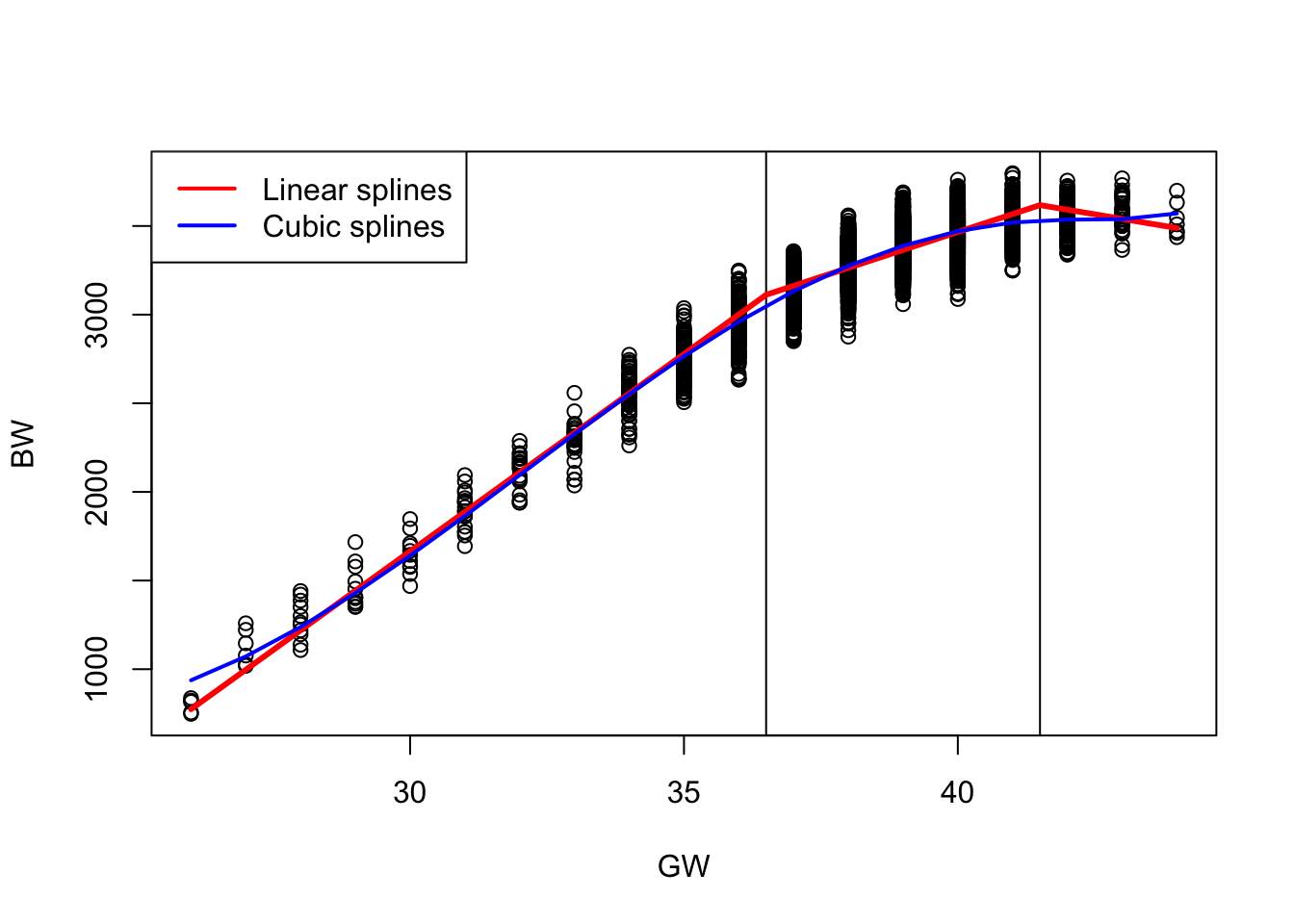

Important

Polynomial Splines

The general formulation of a d-degree polynomial spline model with $M$ knots $k_{1}, k_{2}, k_{3}, . . ., k_{M}$ is

$y_{i} = β_{0} + \sum_{j = 1}^{d} β_{j} x_{i}^{(j)} + \sum_{m = 1}^{M} β_{d + m} (x_{i} - k_{m})_{+}^{d}$

the above is known as the truncated power formulation.
Linear $d = 1$

$y_{i} = β_{0} + β_{1} x_{i} + \sum_{m = 1}^{M} β_{1 + m} (x_{i} - k_{m})_{+}$ - Quadratic $d = 2$

$y_{i} = β_{0} + β_{1} x_{i} + + β_{2} x_{i}^{2} + \sum_{m = 1}^{M} β_{2 + m} (x_{i} - k_{m})_{+}^{2}$

Linear splines are a good choice for interpretability - the coefficients at the knots represent the change in slope from previous region.
Cubic splines appear smooth, which is often biologically reasonable. Generally, we do not interpret the individual coeffs of the truncated polynomials.

summary(fit8)


Call:
lm(formula = bw ~ gw + I(gw^2) + I(gw^3) + Sp1 + Sp2, data = dat)

Residuals:
    Min      1Q  Median      3Q     Max 
-399.13  -74.61    4.47   77.06  301.40 

Coefficients:
              Estimate Std. Error t value Pr(>|t|)    
(Intercept)  2.890e+04  3.717e+03   7.776 9.02e-15 ***
gw          -2.968e+03  3.335e+02  -8.901  < 2e-16 ***
I(gw^2)      9.972e+01  9.900e+00  10.073  < 2e-16 ***
I(gw^3)     -1.036e+00  9.734e-02 -10.641  < 2e-16 ***
Sp1          7.732e-01  2.482e-01   3.115  0.00185 ** 
Sp2          7.455e+00  3.471e+00   2.148  0.03177 *  
---
Signif. codes:  0 '***' 0.001 '**' 0.01 '*' 0.05 '.' 0.1 ' ' 1

Residual standard error: 109.8 on 4994 degrees of freedom
Multiple R-squared:  0.881, Adjusted R-squared:  0.8809 
F-statistic:  7397 on 5 and 4994 DF,  p-value: < 2.2e-16

Basis Splines (B-Splines)

Goal: Find a flexible function $μ (x)$ for the model:

$\begin{aligned} y & = μ (x) + ϵ, ϵ \sim N (0, σ^{2}) \\ μ (x) & = \sum_{k = 1}^{K} β_{k} \cdot b_{k} (x) \\ μ_{i} & = B_{i} β \end{aligned}$

where $B_{i, 1 : K} = (v 1 (x_{i}), b 2 (x_{i}), . . ., b_{k} (x_{i}))$ .

We consider B-splines (basis splines) to model $μ (x)$ . Where $μ (x)$ is a linear combination of basis functions. (A broader family of splines)
B-splines have nice properties and are computationally convenient because they are non-zero on a limited range only.
Computationally more accurate- avoid overflow errors.
Provide better numerical stability.
Any spline function of given degree can be expressed as a linear combination of B-splines of that degree.

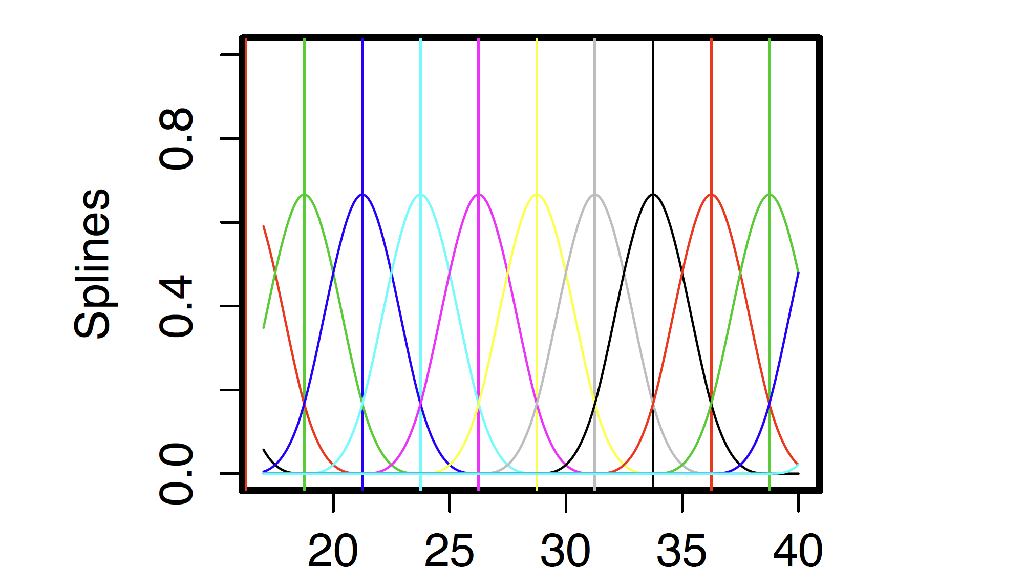
Example of B-Splines

Define a set of knots or breakpoints (of the x-axis), denoted by:

$τ_{1} < τ_{2} < \dots < τ_{g};$

Knot placement is determined in advance. Want them close enough together to capture true fluctuations in $x$ . An example above is equally spaced knots.
A cubic B-spline $b_{k} (x)$ is:
- a piecewise polynomial function of degree $d = 3$ in variable $x$ ;
- non-zero for a range $τ_{k - 2} \leq x \leq τ_{k + 2}$ ;
- at its maximum at knot $τ_{k}$ .

For each $x_{i}$ :

$x_{i} : \sum_{k = 1}^{K} b_{k} (x_{i}) = 1$

B-splines and computation

The $b s ()$ function in R will create the design matrix

library(splines)
set.seed(123)
Blinear = bs(dat$gw, knots = c(36.5, 41.5), degree=1) #basis matrix where each column represents piecewise linear basis functions.
  #Each row. = obs of GW and each column = one linear BF
Bquad = bs(dat$gw, knots = c(36.5, 41.5), degree=2)
Bcubic = bs(dat$gw, knots = c(36.5, 41.5), degree=3)

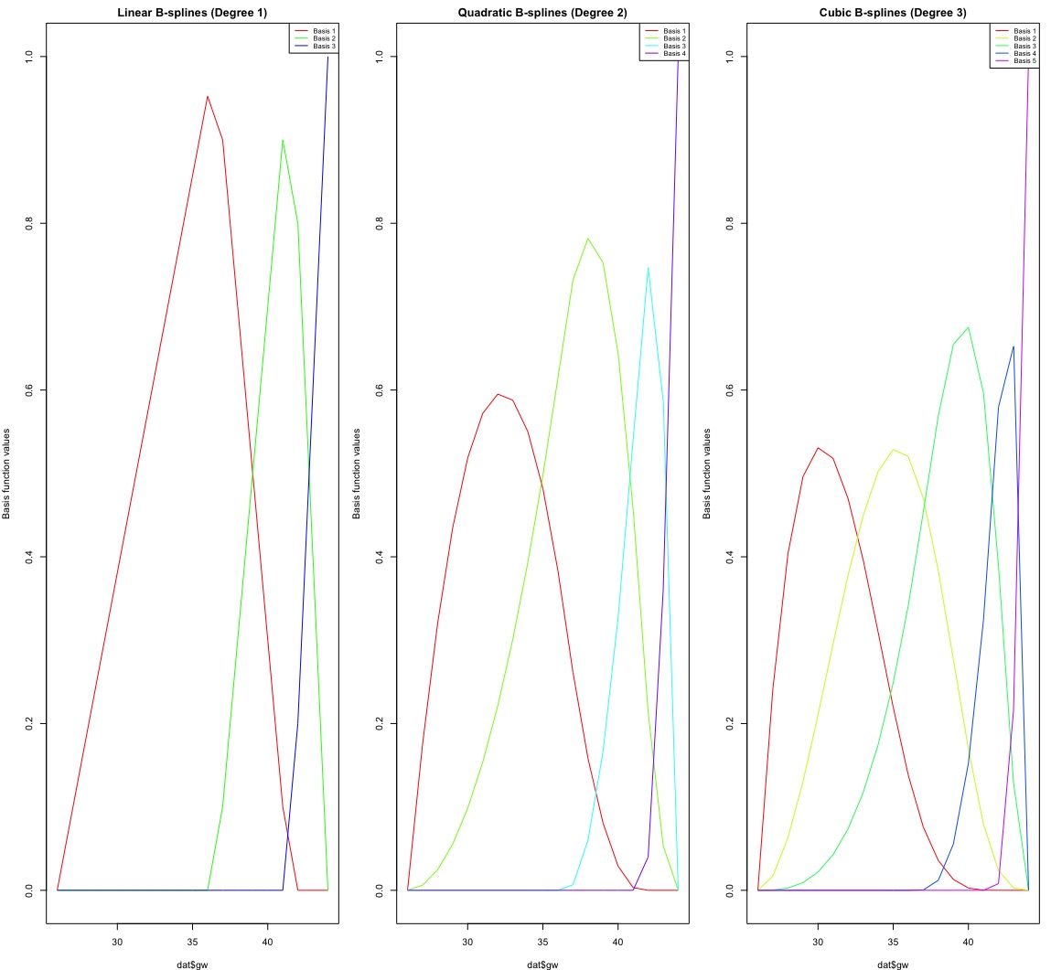
Summary:

Linear B-Splines (Degree 1):
- Piecewise straight lines.
- 3 basis functions (one for each interval between knots).
- Less flexibility, only changes slope at the knots.
Quadratic B-Splines (Degree 2):
- Piecewise parabolas (curved lines).
- 4 basis functions.
- Smoother than linear, with a continuous slope at the knots.
Cubic B-Splines (Degree 3):
- Piecewise cubic curves.
- 5 basis functions.
- Even smoother, with continuous slope and curvature at the knots.

    #Linear splines
    fit1 <- lm(bw ~ bs(gw, knots = c(36.5, 41.5), degree=1), data = dat)
    #Quadratic splines
    fit2 <- lm(bw ~ bs(gw, knots = c(36.5, 41.5), degree=2), data = dat)
    #Cubic splines
    fit3 <- lm(bw ~ bs(gw, knots = c(36.5, 41.5), degree=3), data = dat)

    summary(fit3)


Call:
lm(formula = bw ~ bs(gw, knots = c(36.5, 41.5), degree = 3), 
    data = dat)

Residuals:
    Min      1Q  Median      3Q     Max 
-399.13  -74.61    4.47   77.06  301.40 

Coefficients:
                                           Estimate Std. Error t value Pr(>|t|)
(Intercept)                                  937.45      34.65  27.056  < 2e-16
bs(gw, knots = c(36.5, 41.5), degree = 3)1   408.19      57.92   7.048 2.07e-12
bs(gw, knots = c(36.5, 41.5), degree = 3)2  2037.52      32.46  62.779  < 2e-16
bs(gw, knots = c(36.5, 41.5), degree = 3)3  2655.45      38.15  69.608  < 2e-16
bs(gw, knots = c(36.5, 41.5), degree = 3)4  2582.17      35.94  71.851  < 2e-16
bs(gw, knots = c(36.5, 41.5), degree = 3)5  2633.37      52.76  49.912  < 2e-16
                                              
(Intercept)                                ***
bs(gw, knots = c(36.5, 41.5), degree = 3)1 ***
bs(gw, knots = c(36.5, 41.5), degree = 3)2 ***
bs(gw, knots = c(36.5, 41.5), degree = 3)3 ***
bs(gw, knots = c(36.5, 41.5), degree = 3)4 ***
bs(gw, knots = c(36.5, 41.5), degree = 3)5 ***
---
Signif. codes:  0 '***' 0.001 '**' 0.01 '*' 0.05 '.' 0.1 ' ' 1

Residual standard error: 109.8 on 4994 degrees of freedom
Multiple R-squared:  0.881, Adjusted R-squared:  0.8809 
F-statistic:  7397 on 5 and 4994 DF,  p-value: < 2.2e-16

Interpretation:

Role of Coefficients:
- In a spline model, the estimated coefficients $β_{k}$ represent the contribution of each B-spline basis function $b_{k} (x)$ to the overall predicted value of the response variable $μ (x)$ .
- Each coefficient $β_{k}$ adjusts the height and influence of its corresponding B-spline function across the range of $x$ .
Effect on the Prediction:
- The overall model prediction $μ (x)$ is a linear combination of the B-spline basis functions weighted by their respective coefficients. Thus, the predicted value at a given $x$ is influenced by the specific values of these coefficients and the corresponding basis functions evaluated at $x$ .
Local Interpretation:
- The interpretation of a specific coefficient $β_{k}$ s often local rather than global:
  - If $α_{k}$ is positive, it indicates that the B-spline function $b_{k} (x)$ contributes positively to the predicted value of $μ (x)$ in the range where $b_{k} (x)$ is non-zero.
  - If $α_{k}$ is negative, it implies a negative contribution from $b_{k} (x)$ in its active range.
Influence of Knots:
- The placement of knots influences the shape of the spline and, consequently, how the coefficients interact with the data:
  - The regions between knots allow for changes in the slope and curvature of the spline. Thus, the coefficients can be seen as controlling the smooth transitions between these segments.

Example: Daily Death Counts in NYC

Daily non-accidental mortality counts in 5-county NYC 2001-2006

load(paste0(getwd(), "/data/NYC.RData"))

fit1 = lm (alldeaths~bs (date, df = 10, degree = 1), data = health)
fit2 = lm (alldeaths~bs (date, df = 10, degree = 2), data = health)
fit3 = lm (alldeaths~bs (date, df = 10, degree = 3), data = health)


# NOTE: To see where knots are
temp = bs(health$date,df=10,degree=1) # allows 9 knots; bs does not create column of ones... 
# bs(health$date,df=10,degree=2) # allows 8 knots
# bs(health$date,df=10,degree=3) # allows 7 knots




plot (health$alldeaths~health$date, col = "grey", xlab = "Date", ylab = "Death", main = "Knots at quantiles, df = 10")
lines (fit1$fitted~health$date, col = 2, lwd = 3)
lines (fit2$fitted~health$date, col = 4, lwd = 3)
lines (fit3$fitted~health$date, col = 5, lwd = 3)
legend ("topleft", legend=c("Linear splines", "Quadratic splines", "Cubic splines"), col=c(2,4, 5), lwd=3, cex = 1.3, bty= "n")

fit1 = lm (alldeaths~bs (date, df = 20, degree = 1), data = health)
fit2 = lm (alldeaths~bs (date, df = 20, degree = 2), data = health)
fit3 = lm (alldeaths~bs (date, df = 20, degree = 3), data = health)

plot (health$alldeaths~health$date, col = "grey", xlab = "Date", ylab = "Death", main = "Knots at quantiles, df = 20")
lines (fit1$fitted~health$date, col = 2, lwd = 3)
lines (fit2$fitted~health$date, col = 4, lwd = 3)
lines (fit3$fitted~health$date, col = 5, lwd = 3)
 legend ("topleft", legend=c("Linear splines", "Quadratic splines", "Cubic splines"), col=c(2,4, 5), lwd=3, cex = 1.3, bty= "n")

Model Selection

We need to pick:
- Which basis function? Linear versus Cubic
- How many knots?
- Where to put the knots?

Main Ideas

Choice of basis function usually does not have a large impact on model fit, especially when there are enough knots and $g (x)$ is smooth.
When there are enough knots, their locations are less important too! By “enough” this means distance between them is small enough to capture fluctuations.
So how many knots? is the question.

Important

Bias- Variance Tradeoff

More knots->
- can better capture fine scale trends
- Need to estimate more coefficients (risk of overfitting)
- Below shows cubic splines with different number of knots.

Assume $Y$ comes from some true model.

$Y = g (X) + ϵ, ϵ \sim (0, σ^{2})$

where $g ()$ is some unknown function.
For a given $x_{i}$ , we estimate $Y$ with $\hat{g} (x_{i})$ where here we assume $g (x) ⊥ ϵ$
The expected squared difference between $Y$ and $\hat{g} (x)$ is the population mean squared error (MSE):

MSE = $E [Y - \hat{g} (x)]^{2} = σ^{2} + E [g (x_{i}) - \hat{g} (x_{i})]^{2} = {Bias}^{2} + Variance$
We want to minimize the population MSE, but it is made up of 2 components.

Cross-Validation Error

Let ${\hat{g}}^{(- i)}$ be the fitted value of $y_{i}$ at $x_{i}$ using all the data except $y_{i}$ . The ordinary leave-one-out cross-validation (LOOCV) is given by

$C V = \frac{1}{n} \sum_{i = 1}^{n} (y_{i} - {\hat{g}}^{(- i)} (x_{i}))^{2}$

Intuitively, $C V$ estimates the population Mean Squared Error (MSE), $E [(Y - \hat{g} (X))^{2}]$ , with a sample MSE.

Note here we are averaging across the values of $x_{i}$ .

We want to pick a model that minimizes CV!

Caveat from Hastie et al:
“Discussions of error rate estimation can be confusing, because we have to make clear which quantities are fixed and which are random…”

Overfitting

If you overfit, then you start to fit the noise in the data, i.e., you estimate $g (x_{i}) + ϵ_{i}$ , instead of $g (x_{i})$ .
With overfitting, new data are poorly predicted.

From Bias-Variance perspective:

In splines, lines that are very wiggly = high variance.
If you underfit, then you tend to estimate a smoothed version of $g (x_{i})$ , and at the extreme, fit a mean such that $\hat{g} (x_{i}) = {\bar{y}}_{i}$ .

From Bias-Variance perspective:

In splines, lines that vary little = low variance.