Module 4: Generalized Estimating Equations

Reading

• A useful reference: Halekoh, I., S. Hojsgaard, and J. Yan. The R Package geepack for Generalized Estimating Equations. Journal of Statistical Software. 2006.

• Informal Overview: https://rlbarter.github.io/Practical-Statistics/2017/ 05/10/generalized-estimating-equations-gee/

Basic Concepts

• Weighted and generalized least squares.
• Estimating equation.
• Marginal correlation structures.
• Robust standard error.

Important

Generalized Estimating Equations

• Generalized Estimating Equations (GEEs) are a statistical technique used primarily for analyzing correlated data, such as repeated measures or clustered observations.

Key Features:

1. Population-Averaged Estimates: GEEs focus on estimating the average effects across all subjects rather than individual-level effects.

2. Handling Correlation: GEEs are designed to handle correlated data, such as measurements taken from the same subject over time or from subjects within the same group. GEEs provide more robust estimates and standard errors.

3. Flexibility: GEEs can be applied to various types of data, including binary, count, and continuous outcomes.

4. Robustness: One of the strengths of GEEs is their ability to produce valid statistical inferences even when the specified correlation structure is incorrect.

Motivating Example

Consider data $y_1,y_2$ and $y_3$ from

$$\mathbf{y}=\left(\begin{array}{c}{y}_1\\ y_2\\ y_3\end{array}\right)\sim N(\left(\begin{array}{c}\mu \\ \mu \\ \mu \end{array}\right),\mathrm{\Sigma }=\left(\begin{array}{ccc}{\sigma }^2& R& 0\\ R& {\sigma }^2& 0\\ 0& 0& {\sigma }^2\end{array}\right))$$

• $y_1$ and $y_2$ come from the same cluster and may be correlated, i.e.,

  $$R\ne 0\text{ between }{y}_1\text{ and }{y}_2$$

• $y_1,y_2,y_3$ have the same expectation $\mu$. The average of $y_i$ will give an unbiased estimator.

  $$\hat{\mu }=\frac{y_1+y_2+y_3}{3}$$

• This assigns equal weight, i.e., $a=(1/3,1/3,1/3)$.

• To find the variance-covariance note $cov(aTy)=a^T\{cov(y)\}a$.

• The above estimator has variance given by

  $$[1/3,1/3,1/3]\mathrm{\Sigma }\left[\begin{array}{c}1/3\\ 1/3\\ 1/3\end{array}\right]=\frac{3{\sigma }^2+2R}{9}$$

• As R increases, variance also increases

• Our aim is to find a set of weights $\mathbf{w}=(w_1,w_2,w_3)$ such that:

  $$\hat{\mu }=w_1{y}_1+w_2{y}_2+w_3{y}_3,\text{ where }{w}_i>0\text{ and }\sum _i{w}_i=1$$

• $\hat{\mu }$ is unbiased

• What is the variance for $\hat{\mu }$?

• When $R=0$, minimum variance when $w_1=w_2=w_3$ (the simple sample average).

Consider the following set of weights:

1. Simple average: $\mathbf{w}=(1/3,1/3,1/3)$.
2. Average $y_1$ and $y_2$ first; then average with $y_3$: $\mathbf{w}=(1/4,1/4,1/2)$.
3. Use only one of $y_1$ or $y_2$: $\mathbf{w}=(1/2,0,1/2)$.
4. Secret: assuming $R$ and ${\sigma }^2$ are known: $\mathbf{w}=(\frac{1}{3+R/{\sigma }^2},\frac{1}{3+R/{\sigma }^2},\frac{1+R/{\sigma }^2}{3+R/{\sigma }^2})$.

Estimator Weights	$Var(\hat{\mu })$	$R=0$	$R=0.5{\sigma }^2$	$R={\sigma }^2$
(1/3, 1/3, 1/3)	$\frac{3{\sigma }^2+2R}{9}$	$\frac{1}{3}{\sigma }^2$	$\frac{4}{9}{\sigma }^2$	$\frac{5}{9}{\sigma }^2$
(1/4, 1/4, 1/2)	$\frac{3{\sigma }^2+R}{8}$	$\frac{3}{8}{\sigma }^2$	$\frac{7}{16}{\sigma }^2$	$\frac{1}{2}{\sigma }^2$
(1/2, 0, 1/2)	$\frac{{\sigma }^2}{2}$	$\frac{1}{2}{\sigma }^2$	$\frac{1}{2}{\sigma }^2$	$\frac{1}{2}{\sigma }^2$
$(\frac{1}{3+R/{\sigma }^2},\frac{1}{3+R/{\sigma }^2},\frac{1+R/{\sigma }^2}{3+R/{\sigma }^2})$	$\left(\frac{1+R/{\sigma }^2}{3+R/{\sigma }^2}\right){\sigma }^2$	$\frac{1}{3}{\sigma }^2$	$\frac{3}{7}{\sigma }^2$	$\frac{1}{2}{\sigma }^2$

The secret (optimal) weights

• have the smallest standard error for the complete range of $R$ values.

• become a simple average when $R=0$ (independence).

• gives weight 1/4 to $y_1$ and $y_2$ when $R={\sigma }^2$.

Estimating Equations

All four estimators $\hat{\mu }$ are solutions to the estimating equation. We will define an equation to produce a class of unbiased estimators of $\hat{\mu }$.

We know $E(y_i-\hat{\mu })=0$ for all $i=1,2,3$.

Combining the three equations, an unbiased estimator $\hat{\mu }$ can be obtained by solving:

$$\sum _i{\alpha }_i(y_i-\hat{\mu })=0$$ The above gives:

$$\hat{\mu }=\frac{{\alpha }_1{y}_1+{\alpha }_2{y}_2+{\alpha }_3{y}_3}{{\alpha }_1+{\alpha }_2+{\alpha }_3}$$

Therefore, the weights for $i=1,2,3$ are

$$w_i=\frac{{\alpha }_i}{\sum _i{\alpha }_i}$$

An estimating equation is a very general approach. Equation (1) is an example where we set up an equation, set it to zero, and solve for $\hat{\mu }$. Methods of moments and maximum likelihood (setting the 1st deriv of the log-lik to zero) are examples of estimating equations.

Important

An estimating equation is a mathematical expression used to derive parameter estimates in statistical models. Unlike methods that maximize likelihoods (e.g., maximum likelihood estimation), estimating equations focus on finding parameters that satisfy certain conditions.

Key Features:

• Estimating equations often arise in generalized estimating equations (GEE), which are commonly used to handle correlated data, like repeated measures or clustered data.

• The solution to an estimating equation gives the parameter estimates that “best” explain the observed data, based on the chosen model.

• These equations are particularly useful when the likelihood function is complex or unknown.

Regression with Heteroscedastic Errors

Now consider the linear regression problem with heteroscedastic errors:

$$\mathbf{y}=\mathbf{X}\beta +ϵ,ϵ\sim N(0,\mathbf{V})$$

Here we assume the residual covariance matrix $\mathbf{V}$ is known and diagonal.

$$V=\left[\begin{array}{cccc}{v}_1& 0& ...& 0\\ 0& v_2& ...& 0\\ ⋮& \ddots & \ddots & ⋮\\ 0& ...& ...& v_n\end{array}\right]$$

How can we find the least squares estimate of $\beta$?

Weighted Least Squares

In WLS, we extend the methods we learned in regular OLS to account for heteroscedasticity (unqeual variance) . Each observation is given a weight based on how much reliability we place on it. This allows a better fit to data where some points have more variability than others.

• let $\mathbf{W}$ be a diagonal matrix with $diag(\mathbf{W})=(v_1^{-1/2},v_2^{-1/2},\dots ,v_n^{-1/2})$. Notand e that $\mathbf{W}\mathbf{W}={\mathbf{V}}^{-1}$.

• Now consider the transformed $y$ and transformed $X^{\ast }$:

$$\begin{array}{rl}{\mathbf{y}}^{\mathbf{\ast }}& =\mathbf{W}y\\ {\mathbf{X}}^{\mathbf{\ast }}& =\mathbf{W}\mathbf{X}\end{array}$$

• We now have a regression problem with EQUAL variance:

$$\begin{array}{rl}{\mathbf{y}}^{\mathbf{\ast }}& ={\mathbf{X}}^{\mathbf{\ast }}\beta +{ϵ}^{\mathbf{\ast }},ϵ\mathbf{\ast }\sim N(0,I)\\ \mathbf{Wy}& =\mathbf{WX}\beta +\mathbf{W}ϵ\end{array}$$

• Reminder the OLS estimator $=(X^{T}X{)}^{-1}{X}^{T}y$.

• Derive the weighted least squares estimator for $\beta$, i.e., ${\hat{\beta }}_{WLS}$.

• The WLS estimate is unbiased (for ANY $\mathbf{V}$).

$$\begin{array}{rl}E({\hat{\beta }}_{WLS})& =E(({\mathbf{X}}^T{\mathbf{V}}^{-1}\mathbf{X}{)}^{-1}{\mathbf{X}}^T{\mathbf{V}}^{-1}\mathbf{y})\\ & =({\mathbf{X}}^T{\mathbf{V}}^{-1}\mathbf{X}{)}^{-1}{\mathbf{X}}^T{\mathbf{V}}^{-1}\mathbf{X}\beta \\ & =\beta \end{array}$$ - What if we used regular ordinary least squares estimate?

$$\begin{array}{rl}E({\hat{\beta }}_{OLS})& =E(({\mathbf{X}}^T\mathbf{X}{)}^{-1}{\mathbf{X}}^T\mathbf{y})\\ & =({\mathbf{X}}^T\mathbf{X}{)}^{-1}{\mathbf{X}}^T\mathbf{X}\beta \\ & =\beta \end{array}$$

Still unbiased!

• The OLS estimator of $\beta$ is still unbiased and it is also consistent. So what is the problem?

1. Inference: p-values will be wrong.

2. Efficiency: we can define an estimator with lower variance.

What does this mean?

• The estimate of the covariance for ${\hat{\beta }}_{OLS}$ is given by $({\mathbf{X}}^{\prime }\mathbf{X}{)}^{-1}{\hat{\sigma }}_{OLS}^2$.

• We found the WLS covariance to be

  $$cov(\hat{\beta })=({\mathbf{X}}^{\prime }\mathbf{X}{)}^{-1}{\mathbf{X}}^{\prime }\mathbf{V}\mathbf{X}({\mathbf{X}}^{\prime }\mathbf{X}{)}^{-1}$$

• Then if $\mathbf{V}\ne {\sigma }^{2}I$ the OLS covariance is not correct, i.e., inference is incorrect.

Summary I

• The OLS estimate of the SE of ${\hat{\beta }}_{OLS}$ can lead to invalid inference.
• The true variance of ${\hat{\beta }}_{OLS}$ is larger than ${\hat{\beta }}_{WLS}$ so OLS is inefficient. WLS improves accuracy.

Example: Fixed Effect Meta Analysis

Let ${\hat{\beta }}_i$ be the effect size from study $i$ with estimated variance ${\hat{\sigma }}_i^2$. We will assume the model

$${\hat{\beta }}_i=\mu +{ϵ}_i\text{ where }{ϵ}_i\sim N(0,{\hat{\sigma }}_i^2)$$ This can be expressed as:

$$\begin{array}{rl}\mathbf{y}& =[{\hat{\beta }}_1,{\hat{\beta }}_2,...,{\hat{\beta }}_n{]}^{\prime }\\ \mathbf{X}& =[1,1,...,1{]}^{\prime }\text{ (i.e., intercept only)}\\ \mathbf{V}& =diag({\hat{\sigma }}_1^2,...,{\hat{\sigma }}_n^2)\end{array}$$

Therefore:

• ${\mathbf{V}}^{-1}=diag(1/{\hat{\sigma }}_1^2,{\hat{\sigma }}_2^2,...,{\hat{\sigma }}_n^2)$.
• ${\mathbf{X}}^{\prime }{\mathbf{V}}^{-1}=(1/{\hat{\sigma }}_1^2,{\hat{\sigma }}_2^2,...,{\hat{\sigma }}_n^2)$
• ${\mathbf{X}}^{\prime }{\mathbf{V}}^{-1}\mathbf{V}=\sum _{i=1}^{n}1/{\hat{\sigma }}_i^2$
• ${\mathbf{X}}^{\prime }{\mathbf{V}}^{-1}\mathbf{y}=\sum _{i=1}^n{\hat{\beta }}_i/{\hat{\sigma }}_i^2$

$${\mu }_{WLS}=({\mathbf{X}}^{\prime }{\mathbf{V}}^{-1}\mathbf{X}{)}^{-1}{\mathbf{X}}^{\prime }{\mathbf{V}}^{-1}\mathbf{y}=\frac{\sum _{i=1}^n{\hat{\beta }}_i/{\hat{\sigma }}_i^2}{\sum _{i=1}^{n}1/{\hat{\sigma }}_i^2}$$ the inverse-variance weighted average!.

• What do we do if $\mathbf{V}$ is not diagonal, meaning the errors are not independent?

Generalized Least Squares

• For non-diagonal $\mathbf{V}$, this means that the errors are not independent. So there is heteroscedasticity (non-constant variance) AND correlated errors.

$${\hat{\beta }}_{GLS}=({\mathbf{X}}^{\prime }{\mathbf{V}}^{-1}\mathbf{X}{)}^{-1}{\mathbf{X}}^{\prime }{\mathbf{V}}^{-1}\mathbf{y}$$

Derivation of the covariance, i.e., $cov({\hat{\beta }}_{GLS})$:

1. Error Structure: We assume that the error term $(ϵ)$ has the following structure: $$ϵ\sim \mathcal{N}(0,\mathbf{V})$$ where $(\mathbf{V})$ is the variance-covariance matrix of the errors.
2. Substituting $(\mathbf{y})$ into the expression for $({\hat{\beta }}_{GLS}):$

$${\hat{\beta }}_{GLS}=({\mathbf{X}}^{\prime }{\mathbf{V}}^{-1}\mathbf{X}{)}^{-1}{\mathbf{X}}^{\prime }{\mathbf{V}}^{-1}(\mathbf{X}\beta +ϵ)$$ This can be expanded to: $${\hat{\beta }}_{GLS}=({\mathbf{X}}^{\prime }{\mathbf{V}}^{-1}\mathbf{X}{)}^{-1}{\mathbf{X}}^{\prime }{\mathbf{V}}^{-1}\mathbf{X}\beta +({\mathbf{X}}^{\prime }{\mathbf{V}}^{-1}\mathbf{X}{)}^{-1}{\mathbf{X}}^{\prime }{\mathbf{V}}^{-1}ϵ$$ The first term simplifies to $(\beta )$: ${\hat{\beta }}_{GLS}=\beta +({\mathbf{X}}^{\prime }{\mathbf{V}}^{-1}\mathbf{X}{)}^{-1}{\mathbf{X}}^{\prime }{\mathbf{V}}^{-1}ϵ$

4. To find the covariance of $({\hat{\beta }}_{GLS})$, we need the covariance of the error term. The error term $(ϵ)$ is zero-mean and has variance-covariance matrix $(\mathbf{V})$:

$$\text{Cov}({\hat{\beta }}_{GLS})=\text{Cov}(({\mathbf{X}}^{\prime }{\mathbf{V}}^{-1}\mathbf{X}{)}^{-1}{\mathbf{X}}^{\prime }{\mathbf{V}}^{-1}ϵ)$$ Using the property that $(\text{Cov}(A\mathbf{Z})=A\text{Cov}(\mathbf{Z})A^{\prime })$ for any constant matrix $(A)$ and random vector $(\mathbf{Z}):$
$$\text{Cov}({\hat{\beta }}_{GLS})=({\mathbf{X}}^{\prime }{\mathbf{V}}^{-1}\mathbf{X}{)}^{-1}{\mathbf{X}}^{\prime }{\mathbf{V}}^{-1}\text{Cov}(ϵ){\mathbf{V}}^{-1}\mathbf{X}({\mathbf{X}}^{\prime }{\mathbf{V}}^{-1}\mathbf{X}{)}^{-1}$$ Substituting $(\text{Cov}(ϵ)=\mathbf{V})$: $$\text{Cov}({\hat{\beta }}_{GLS})=({\mathbf{X}}^{\prime }{\mathbf{V}}^{-1}\mathbf{X}{)}^{-1}{\mathbf{X}}^{\prime }{\mathbf{V}}^{-1}\mathbf{V}{\mathbf{V}}^{-1}\mathbf{X}({\mathbf{X}}^{\prime }{\mathbf{V}}^{-1}\mathbf{X}{)}^{-1}$$ This simplifies to: $$\text{Cov}(\hat{\beta }GLS)=({\mathbf{X}}^{\prime }{\mathbf{V}}^{-1}\mathbf{X}{)}^{-1}{\mathbf{X}}^{\prime }{\mathbf{V}}^{-1}\mathbf{X}({\mathbf{X}}^{\prime }{\mathbf{V}}^{-1}\mathbf{X}{)}^{-1}$$ Finally, since the middle terms cancel out: $$\text{Cov}({\hat{\beta }}_{GLS})=({\mathbf{X}}^{\prime }{\mathbf{V}}^{-1}\mathbf{X}{)}^{-1}$$

Generalized Least Squares: Homoscedastic

• For a normal (Gaussian) regression model, we often assume the observations are homoscedastic (equal variance). The model can be expressed as:

$$y=\mathbf{X}\beta +ϵ,ϵ\sim N(0,\mathbf{V})$$

where $(\mathbf{V}={\sigma }^2\mathbf{R})$.

• The Generalized Least Squares (GLS) estimator is given by:

$${\hat{\beta }}_{GLS}=({\mathbf{X}}^{\prime }{\mathbf{V}}^{-1}\mathbf{X}{)}^{-1}{\mathbf{X}}^{\prime }{\mathbf{V}}^{-1}\mathbf{y}$$

• Substituting $\mathbf{V}={\sigma }^2\mathbf{R}$ for homoscedasticity, we have:

$${\hat{\beta }}_{GLS}=({\mathbf{X}}^{\prime }{\sigma }^2{\mathbf{R}}^{-1}\mathbf{X}{)}^{-1}{\mathbf{X}}^{\prime }{\sigma }^2{\mathbf{R}}^{-1}\mathbf{y}=({\mathbf{X}}^{\prime }{\mathbf{R}}^{-1}\mathbf{X}{)}^{-1}{\mathbf{X}}^{\prime }{\mathbf{R}}^{-1}\mathbf{y}$$ - The covariance matrix of the GLS estimator is given by:

$$\text{Cov}({\hat{\beta }}_{GLS})=({\mathbf{X}}^{\prime }{\mathbf{V}}^{-1}\mathbf{X}{)}^{-1}=({\mathbf{X}}^{\prime }{\sigma }^2{\mathbf{R}}^{-1}\mathbf{X}{)}^{-1}={\sigma }^2({\mathbf{X}}^{\prime }{\mathbf{R}}^{-1}\mathbf{X}{)}^{-1}$$

• Later on this is called the naive SE in $gee::gee$.

Motivating Example

1. Back to the motivating example assume ${\sigma }^2=1$, the assumed model for the outcome $\mathbf{y}$:

$$\mathbf{y}=\left[\begin{array}{c}{y}_1\\ y_2\\ y_3\end{array}\right]\sim N(\mu ,\left[\begin{array}{ccc}1& R& 0\\ R& 1& 0\\ 0& 0& 1\end{array}\right])$$

where $\mathbf{X}=[1,1,1{]}^{\prime }$.

2. The inverse of the variance-covariance matrix ${\mathbf{V}}^{-1}$ given by:

$${\mathbf{V}}^{-1}=\left[\begin{array}{ccc}\frac{1}{1-R^2}& -\frac{R}{1-R^2}& 0\\ -\frac{R}{1-R^2}& \frac{1}{1-R^2}& 0\\ 0& 0& 1\end{array}\right]$$

3. Calculating $({\mathbf{X}}^{\prime }{\mathbf{V}}^{-1}\mathbf{X}){\mathbf{X}}^{\prime }{\mathbf{V}}^{\mathbf{-}\mathbf{1}}$:

$${\mathbf{X}}^{\prime }{\mathbf{V}}^{-1}\mathbf{X}=[1,1,1]\left[\begin{array}{ccc}\frac{1}{1-R^2}& -\frac{R}{1-R^2}& 0\\ -\frac{R}{1-R^2}& \frac{1}{1-R^2}& 0\\ 0& 0& 1\end{array}\right]\left[\begin{array}{c}1\\ 1\\ 1\end{array}\right]=\frac{3-2R-R^2}{1-R^2}=\frac{(3+R)(1-R)}{(1-R)(1+R)}=\frac{3+R}{1+R}$$

4. The inverse of ${\mathbf{X}}^{\prime }{\mathbf{V}}^{-1}\mathbf{X}$:

$${\left({\mathbf{X}}^{\prime }{\mathbf{V}}^{-1}\mathbf{X}\right)}^{-1}{\mathbf{X}}^{\prime }{\mathbf{V}}^{-1}=\frac{1+R}{3+R}\left[\begin{array}{c}\frac{1}{1+R},\frac{1}{1+R},1\end{array}\right]=\left[\begin{array}{c}\frac{1}{3+R},\frac{1}{3+R},\frac{1+R}{3+R}\end{array}\right]=\text{ secret weights}$$

Generalized Least Squares: Robust Regression

Handling Unknown Variance-Covariance Matrix

If we know $\mathbf{V}$ and $\mathbf{V}\ne {\sigma }^2\mathbf{I}$, we have:

$$y=\mathbf{X}\beta +ϵ,ϵ\sim N(0,\mathbf{V}).$$

The generalized least squares estimate ${\hat{\beta }}_{GLS}$:

• Accounts for the correlation between observations, resulting in an estimator with lower variance.
• The variance $({\mathbf{X}}^{\prime }{\mathbf{V}}^{-1}\mathbf{X}{)}^{-1}$ allows for valid inference.

However, what if $\mathbf{V}$ is unknown (as is often the case)?

Initial Approach:

• Use the Ordinary Least Squares (OLS) estimator:

$${\hat{\beta }}_{OLS}=({\mathbf{X}}^{\prime }\mathbf{X}{)}^{-1}{\mathbf{X}}^{\prime }\mathbf{y}$$ because it is unbiased and consistent.

However,when heteroskedasticity is present,OLS estimates of standard errors may be biased. To correct for this, we use robust standard errors, also known as the sandwich estimator.

Robust Standard Error

For standard errors, recall:

$$\text{Cov}({\hat{\beta }}_{OLS})=({\mathbf{X}}^{\prime }\mathbf{X}{)}^{-1}{\mathbf{X}}^{\prime }\mathbf{V}\mathbf{X}({\mathbf{X}}^{\prime }\mathbf{X}{)}^{-1}$$

So we can estimate $\mathbf{V}$ and plug it in:

$$\widehat{cov}({\hat{\beta }}_{OLS})=({\mathbf{X}}^{\prime }\mathbf{X}{)}^{-1}{\mathbf{X}}^{\prime }\hat{\mathbf{V}}\mathbf{X}(X^{\prime }X{)}^{-1}$$

• One estimate of $\hat{\mathbf{V}}$ is simply the empirical residual covariance:

$$\begin{array}{rl}\widehat{\hat{\mathbf{V}}}& =[\mathbf{y}-\mathbf{X}{\hat{\beta }}_{OLS}][\mathbf{y}-\mathbf{X}{\hat{\beta }}_{OLS}{]}^{\prime }\\ & =\left(\begin{array}{ccc}(y_1-x_1^{{}^{\prime }}{\hat{\beta }}_{OLS}{)}^2& (y_1-x_1^{{}^{\prime }}{\hat{\beta }}_{OLS})(y_2-x_2^{{}^{\prime }}{\hat{\beta }}_{OLS})& \cdots \\ (y_2-x_2^{{}^{\prime }}{\hat{\beta }}_{OLS})(y_1-x_1^{{}^{\prime }}{\hat{\beta }}_{OLS})& (y_2-x_2^{{}^{\prime }}{\hat{\beta }}_{OLS}{)}^2& \cdots \\ ⋮& ⋮& \ddots \end{array}\right)\end{array}$$

Thus, the robust covariance matrix is:

$$\widehat{Cov}({\hat{\beta }}_{OLS}{)}_{\text{robust}}=(X^{\prime }X{)}^{-1}{X}^{\prime }[(y-X{\hat{\beta }}_{OLS})(y-X{\hat{\beta }}_{OLS}{)}^{\prime }]X(X^{\prime }X{)}^{-1}$$

Important

This is commonly referred to as the sandwich estimator because of its “bread-meat-bread” structure, with the covariance matrix being “sandwiched” between terms involving the design matrix $X$.

• The robust standard error provides an estimate of the covariance matrix $cov(\hat{\beta })$ given by:

$$\widehat{Cov}({\hat{\beta }}_{OLS}{)}_{\text{robust}}=(X^{\prime }X{)}^{-1}{X}^{\prime }[(y-X{\hat{\beta }}_{OLS})(y-X{\hat{\beta }}_{OLS}{)}^{\prime }]X(X^{\prime }X{)}^{-1}$$

• However, the empirical estimate of the “meat” component uses only one observation for each element.

$$(y-X{\hat{\beta }}_{OLS})(y-X{\hat{\beta }}_{OLS}{)}^{\prime }$$

Thus it is a poor estimator of $\mathbf{V}$, i.e., inaccurate. We can have a better estimate if we have some idea about what is the structure of $V$.

Tradeoffs in Modeling

• When assumptions are true:
  • stronger assumptions = more accurate estimates.
  • weaker assumptions = less accurate if there is more structure to exploit.
• When assumptions are false:
  • stronger assumptions = incorrect inference.
  • weaker assumptions = more robust.

For example, we see this is non-parametric tests, which are generally less powerful when parametric assumptions hold.

Simulation Exercise: Robust Standard Errors

In this exercise, you will simulate data with heteroskedasticity, fit an OLS model, and compare the standard errors from the OLS with the robust standard errors using the sandwich estimator.

Objective

• Simulate data where the error variance depends on an explanatory variable (i.e., heteroskedasticity).
• Fit an OLS model to the data.
• Calculate both the usual OLS standard errors and the heteroskedasticity-robust (sandwich) standard errors.
• Observe the differences in the standard errors.

Step 1: Simulate Heteroskedastic Data

We will simulate a dataset where the variance of the error term depends on the value of an independent variable, creating heteroskedasticity.

library(sandwich)
library(lmtest)

Warning: package 'lmtest' was built under R version 4.0.5

Loading required package: zoo

Attaching package: 'zoo'

The following objects are masked from 'package:base':

    as.Date, as.Date.numeric

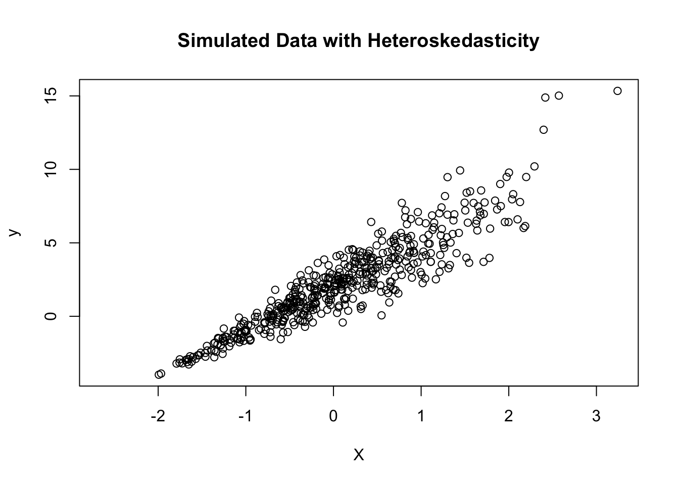
# Set seed for reproducibility
set.seed(123)

# Number of observations
n <- 500

# Generate the independent variable
X <- rnorm(n)

# Generate heteroskedastic errors (variance depends on X)
errors <- rnorm(n, mean = 0, sd = 1 + 0.5 * X)

Warning in rnorm(n, mean = 0, sd = 1 + 0.5 * X): NAs produced

# Generate the dependent variable (y = 2 + 3*X + error)
y <- 2 + 3 * X + errors

# Create a data frame
data <- data.frame(y, X)

# Visualize the data and heteroskedasticity
plot(X, y, main = "Simulated Data with Heteroskedasticity",
     xlab = "X", ylab = "y")

Step 2: Fit an OLS Model

# Fit an OLS model
ols_model <- lm(y ~ X, data = data)

# Summary of the OLS model
summary(ols_model)

Call:
lm(formula = y ~ X, data = data)

Residuals:
    Min      1Q  Median      3Q     Max 
-3.5643 -0.5815  0.0211  0.5905  5.6468 

Coefficients:
            Estimate Std. Error t value Pr(>|t|)    
(Intercept)  1.98200    0.05315   37.29   <2e-16 ***
X            3.00384    0.05734   52.39   <2e-16 ***
---
Signif. codes:  0 '***' 0.001 '**' 0.01 '*' 0.05 '.' 0.1 ' ' 1

Residual standard error: 1.172 on 488 degrees of freedom
  (10 observations deleted due to missingness)
Multiple R-squared:  0.849, Adjusted R-squared:  0.8487 
F-statistic:  2744 on 1 and 488 DF,  p-value: < 2.2e-16

Step 3: Calculate Standard Errors

Next we calculate both the usual OLS SEs and the robust SEs using the $sandwich$ package. You can repeat this simulation with different levels of heteroskedasticity by adjusting the relationship between the variance of the errors and $X$.

# OLS standard errors
ols_se <- sqrt(diag(vcov(ols_model)))

# Robust standard errors (using the HC3 estimator)
robust_se <- sqrt(diag(vcovHC(ols_model, type = "HC3")))

# Display the results
results <- data.frame(
  Coefficient = coef(ols_model),
  OLS_SE = ols_se,
  Robust_SE = robust_se
)
print(results)

            Coefficient     OLS_SE  Robust_SE
(Intercept)    1.981999 0.05315019 0.04920391
X              3.003839 0.05733988 0.07914941

Interpretation:

• Heteroskedasticity Impact: The data was simulated to have heteroskedastic errors.

  • This violates one of the key assumptions of the OLS model—that errors are homoscedastic (i.e., have constant variance).

  • As a result, the OLS standard errors become unreliable (underestimated) when heteroskedasticity is present.

• OLS Standard Errors: These standard errors may be too small, leading to incorrect conclusions about the significance of predictors.

• Robust Standard Errors: The robust (sandwich) standard errors account for heteroskedasticity and provide more accurate estimates of the variability in the coefficient estimates.

  • They adjust for the unequal error variance, resulting in larger standard errors vs OLS.
  • By using robust standard errors, the true variability is captured more accurately, which may increase the standard errors, lowering the t-values and thus reducing the likelihood of falsely identifying significant relationships.
  • The key takeaway is that OLS standard errors cannot be trusted when heteroskedasticity is present. The robust standard errors are a better reflection of the uncertainty in the coefficient estimates in this situation.

Next steps… assuming some structure on $\mathbf{V}$.

Introducing structure to $\mathbf{V}$

Lets call this $\tilde{V}$.

Step 1: Generalized Least Squares (GLS): Use ${\hat{\beta }}_{\text{gls}}=(X^{\prime }{\tilde{V}}^{-1}X{)}^{-1}{X}^{\prime }{\tilde{V}}^{-1}y$ because it is unbiased and consistent

Step 2: Use the sandwich estimator, which adjusts for potential misspecification of $\tilde{V}$. The robust covariance matrix for the GLS estimator is given by:

$$\widehat{\text{Cov}}({\hat{\beta }}_{\text{gls}}{)}_{\text{robust}}=(X^{\prime }{\tilde{V}}^{-1}X{)}^{-1}{X}^{\prime }{\tilde{V}}^{-1}[y-X{\hat{\beta }}_{\text{ols}}]{[y-X{\hat{\beta }}_{\text{ols}}]}^{\prime }{\tilde{V}}^{-1}X(X^{\prime }{\tilde{V}}^{-1}X{)}^{-1}$$ Idea: even if $\tilde{V}$ is misspecified, the SEs are valid for inference (confidence intervals, hypothesis testing)!

If we get the structure correct, we get more accurate estimate of $\beta$.

Summary II

• Heteroskedasticity Correction:
  • OLS assumes homoscedasticity (constant variance of errors). When this assumption is violated (heteroskedasticity), OLS standard errors are biased and unreliable.
  • Robust regression adjusts standard errors to account for heteroskedasticity, providing more reliable inference.
• Robust Standard Errors:
  • Robust standard errors (sandwich estimators), provide a consistent estimate of the variance even when the errors have non-constant variance or are heteroskedastic.
• Bias in OLS Standard Errors:
  • In the presence of heteroskedasticity, OLS tends to underestimate the standard errors, leading to (false positives for significance).
  • Robust standard errors correct this issue, leading to more accurate p-values and confidence intervals.
• Generalization to Misspecified Models:
  • Even if model is misspecified (e.g., the structure of the errors is not correctly modeled), robust SEs yield valid inference.
• Advantages of Robust Regression:
  • Reduces the influence of outliers and high-leverage points that might skew OLS estimates.
  • It is more flexible in the face of violations of assumptions, making it suitable for datasets with heteroskedasticity, outliers, or non-normal error distributions.

Marginal Model for Pig Data

Motivating Example

Let $y_{ij}$ be the weight (kg) at the $jth$ week for the $ith$ pig.

For $i=1,...,48$, $j=1...9$ we wish to model weight as a function of week:

We assume independence between pigs:

$$y_{ij}={\beta }_0+{\beta }_1{x}_{ij}+{ϵ}_{ij}\text{where}{ϵ}_i\sim N(0,{\mathbf{V}}_i)\text{and}{V}_i={\sigma }^2{R}_i(\theta )$$

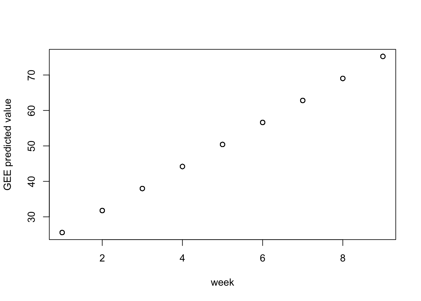
We will estimate ${\beta }_0$ and ${\beta }_1$ using Generalized Estimating Equations (GEE), which is a marginal approach. This differs from the random effects approach in the following ways:

• We do not specify pig-specific intercepts or slopes; instead, we focus on how the within-group data are correlated $R_i(\theta )$.

Advantages:

• The correlation structure $R_i(\alpha )$ can be very flexible.

• Even if we specify $R_i(\alpha )$ incorrectly, we still obtain robust standard errors.

Disadvantages:

• The marginal model does not provide subject-specific predictions since there are no random effects to balance subject-specific information with population information.

• It can be less powerful compared to mixed models.

library(gee)

Warning: package 'gee' was built under R version 4.0.5

library(geepack)

pigdata <- read.csv(paste0(getwd(), "/data/pig.csv"))
  head(pigdata)

  X id weeks weight
1 1  1     1   24.0
2 2  1     2   32.0
3 3  1     3   39.0
4 4  1     4   42.5
5 5  1     5   48.0
6 6  1     6   54.5

fit <-  gee::gee(weight ~ weeks, id = id, data = pigdata, family = "gaussian", corstr = "exchangeable")

Beginning Cgee S-function, @(#) geeformula.q 4.13 98/01/27

running glm to get initial regression estimate

(Intercept)       weeks 
  19.355613    6.209896 

summary(fit)

 GEE:  GENERALIZED LINEAR MODELS FOR DEPENDENT DATA
 gee S-function, version 4.13 modified 98/01/27 (1998) 

Model:
 Link:                      Identity 
 Variance to Mean Relation: Gaussian 
 Correlation Structure:     Exchangeable 

Call:
gee::gee(formula = weight ~ weeks, id = id, data = pigdata, family = "gaussian", 
    corstr = "exchangeable")

Summary of Residuals:
        Min          1Q      Median          3Q         Max 
-11.9050926  -2.5347801  -0.1951968   2.5949074  13.1751157 


Coefficients:
             Estimate Naive S.E.   Naive z Robust S.E. Robust z
(Intercept) 19.355613  0.5983680  32.34734  0.39963854 48.43280
weeks        6.209896  0.0393321 157.88366  0.09107443 68.18485

Estimated Scale Parameter:  19.29006
Number of Iterations:  1

Working Correlation
           [,1]      [,2]      [,3]      [,4]      [,5]      [,6]      [,7]
 [1,] 1.0000000 0.7690313 0.7690313 0.7690313 0.7690313 0.7690313 0.7690313
 [2,] 0.7690313 1.0000000 0.7690313 0.7690313 0.7690313 0.7690313 0.7690313
 [3,] 0.7690313 0.7690313 1.0000000 0.7690313 0.7690313 0.7690313 0.7690313
 [4,] 0.7690313 0.7690313 0.7690313 1.0000000 0.7690313 0.7690313 0.7690313
 [5,] 0.7690313 0.7690313 0.7690313 0.7690313 1.0000000 0.7690313 0.7690313
 [6,] 0.7690313 0.7690313 0.7690313 0.7690313 0.7690313 1.0000000 0.7690313
 [7,] 0.7690313 0.7690313 0.7690313 0.7690313 0.7690313 0.7690313 1.0000000
 [8,] 0.7690313 0.7690313 0.7690313 0.7690313 0.7690313 0.7690313 0.7690313
 [9,] 0.7690313 0.7690313 0.7690313 0.7690313 0.7690313 0.7690313 0.7690313
           [,8]      [,9]
 [1,] 0.7690313 0.7690313
 [2,] 0.7690313 0.7690313
 [3,] 0.7690313 0.7690313
 [4,] 0.7690313 0.7690313
 [5,] 0.7690313 0.7690313
 [6,] 0.7690313 0.7690313
 [7,] 0.7690313 0.7690313
 [8,] 1.0000000 0.7690313
 [9,] 0.7690313 1.0000000

round(fit$working.correlation[1:3, 1:3], 2)

     [,1] [,2] [,3]
[1,] 1.00 0.77 0.77
[2,] 0.77 1.00 0.77
[3,] 0.77 0.77 1.00

Interpretation:

• ${\hat{\beta }}_{week}=6.2$ meaning there is a 6.21 unit change in weight per one unit change in week.

• Naive S.E. shows standard errors of coefficient estimates assuming NO correlation. - Robust S.E. shows shows standard errors of coefficient estimates adjusted for correlation among observations within clusters.

• The Robust SE is higher compared to Naive S.E., 0.09 vs. 0.04, respectively.

• Week is significant using both Naive and Robust methods.

• In GEEs you can only estimate effects averaged across ALL subjects: Meaning GEEs are designed to estimate the avg effects of predictors across all subjects. This is in contrast to mixed models which can estimate both fixed and subject specific effects.

Subject-Specific Predictions

• In GEEs you can only estimate effects averaged across all subject: $y\mathrm{\_}ij={\beta }_0+{\beta }_1{x}_{ij}+ϵij,{ϵ}_i\sim N(0,{\mathbf{V}}_i)$

• Advantages:

  • $R_i(\alpha )$ can be very flexible.

  • Even if we get $R_i(\alpha )$ wrong, we still have robust standard error.

• Disadvantages:

  • Marginal model does not provide subject
  • specific prediction
  • no random effect to balance subject-specific information with population-level information.
  • Can be less powerful than mixed models.

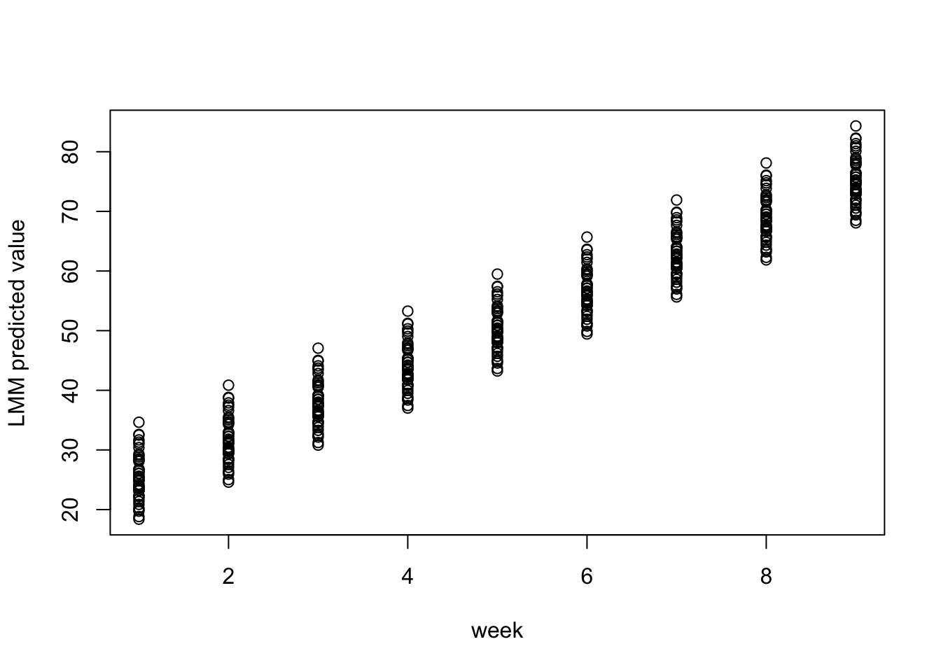
Compared to Random Intercept Model

$$\begin{array}{rl}{y}_{ij}& ={\beta }_0+{\theta }_i+{\beta }_1{x}_{ij}+{ϵ}_{ij},\\ {ϵ}_{ij}& \sim N(0,{\sigma }^2)\\ {\theta }_i& \sim N(0,{\tau }^2)\end{array}$$

library(lme4)

Loading required package: Matrix

fit.mixed <- lmer(weight ~ weeks + (1|id), data = pigdata)
summary(fit.mixed)

Linear mixed model fit by REML ['lmerMod']
Formula: weight ~ weeks + (1 | id)
   Data: pigdata

REML criterion at convergence: 2033.8

Scaled residuals: 
    Min      1Q  Median      3Q     Max 
-3.7390 -0.5456  0.0184  0.5122  3.9313 

Random effects:
 Groups   Name        Variance Std.Dev.
 id       (Intercept) 15.142   3.891   
 Residual              4.395   2.096   
Number of obs: 432, groups:  id, 48

Fixed effects:
            Estimate Std. Error t value
(Intercept) 19.35561    0.60314   32.09
weeks        6.20990    0.03906  158.97

Correlation of Fixed Effects:
      (Intr)
weeks -0.324

• ${\hat{\beta }}_1=6.210$ with $SE=0.039$. Here, equal tp GEE wtih exchangeable working correlation matrix and its naive SE.
• The estimated intra-class correlation is $\frac{15.1}{15.1+4.39}=0.77$, same as the estimated exchangeable working correlation.
• Recall that the random intercept model induces exchanggeable correlation
• Subject prediction in LMMs are more accurate for subject specific predictions.

$$cov(y_{ij},y_{i{j}^{\prime }}={\tau }^2)$$

Extending the definition of GEE for non-normal data

Important

Generalized Estimating Equations

• For normal regression, the GEE approach corresponds nicely to a generalized regression.
• However, GEEs are commonly used to analyze count data, binary outomes, and other data modeled using a distribution from an exponential family.
• GEEs are a general method for analyzing grouped data when:
  • observations within a cluster may be correlated.
  • observations in separate clusters are independent.
  • a monotone transformation of the expectation is linearly related to the explanatory variables, i.e., the link function in GLM.
  • the variance is a function of the expectation. Note: Robust SEs allows for departures from this.

Model Residual Variance in Poisson or Bernoulli Regression

One challenge is that for Poisson or Bernoulli regression, the residual variance depends on the mean structure. For example, consider a logistic regression model. We have:

$$y_i\sim \text{Bernoulli}(p_i)$$

where:

$$p_i=\frac{e^{x_i^0}}{1+e^{x_i^0}}$$

The variance-covariance matrix $V$ is then given by:

$$V=\left[\begin{array}{cccc}\frac{e^{x_1\beta }}{1+e^{x_1\beta }}\cdot \frac{1}{1+e^{x_1\beta }}& 0& \dots & 0\\ 0& \frac{e^{x_2\beta }}{1+e^{x_2\beta }}\cdot \frac{1}{1+e^{x_2\beta }}& \dots & 0\\ ⋮& ⋮& \ddots & ⋮\\ 0& 0& \dots & \frac{e^{x_n\beta }}{1+e^{x_n\beta }}\cdot \frac{1}{1+e^{x_n\beta }}\end{array}\right]$$

• Even without clustering, the marginal covariance has unequal variances that depend on $\beta$.
• To see how GEE work for Generalized Linear Models (GLMs), we need to examine in more detail how these models are fitted.

Revisit GLMs: Estimation for independent data

** Normal Regression**

Consider the linear regression model :

$$y=X\beta +ϵ,ϵ\sim N(0,V).$$

The likelihood function $L(y;\beta )$ is:

$$L(y;\beta )=(2\pi {)}^{-n/2}|V{|}^{-1/2}\exp (-\frac{1}{2}(y-X\beta {)}^t{V}^{-1}(y-X\beta ))$$

If we assume $V$ is diagonal, the data likelihood simplifies to:

$$L(y;\beta )=(2\pi {)}^{-n/2}|V{|}^{-1/2}\exp (-\sum _{i=1}^n\frac{(y_i-x_i^t\beta {)}^2}{v_i})$$

Therefore, the maximum likelihood estimate of $\beta$ can be obtained by minimizing the function:

$$U(\beta )=\sum _{i=1}^n\frac{1}{v_i}(y_i-x_i^t\beta {)}^2.$$

This is equivalent to solving the system of linear equations:

$$\frac{\partial U(\beta )}{\partial \beta }=\sum _{i=1}^n\frac{1}{v_i}{x}_{ik}(y_i-x_i^t\beta )=0$$

The above expression represents an estimating equation too.

** Logistic Regression Model**

$$y_i\sim \text{Bernoulli}(p_i),\text{with}{p}_i=\frac{e^{x_i^t\beta }}{1+e^{x_i^t\beta }}.$$

For a single observation $y_i$, the log-likelihood is given by:

$$l(y_i;\beta )=y_i\cdot x_i^t\beta -\log (1+e^{x_i^t\beta }).$$

The score function is:

$$\frac{\partial l(y_i;\beta )}{\partial {\beta }_k}=x_{ik}{y}_i-\frac{x_{ik}{e}^{x_i^t\beta }}{1+e^{x_i^t\beta }}=x_{ik}(y_i-\frac{e^{x_i^t\beta }}{1+e^{x_i^t\beta }})$$

Therefore, the maximum likelihood estimate (MLE) of $\beta$ is obtained by solving $p$ equations with $p$ unknowns:

$$\sum _{i=1}^n{x}_{ik}(y_i-\frac{e^{x_i^t\beta }}{1+e^{x_i^t\beta }})=0$$

** Poisson Regression**

$$y_i\sim \text{Poisson}({\lambda }_i),\text{with}{\lambda }_i=e^{x_i^t\beta }.$$

For a single observation $y_i$, the log-likelihood is given by:

$$l(y_i;\beta )=-e^{x_i^t\beta }+y_i\cdot x_i^t\beta -\log (y_i!).$$

The score function with respect to ${\beta }_k$ is:

$$\frac{\partial l(y_i;\beta )}{\partial {\beta }_k}=-x_{ik}{e}^{x_i^t\beta }+y_i{x}_{ik}=x_{ik}(y_i-e^{x_i^t\beta }).$$

Therefore, the MLE of $\beta$ is obtained by solving a system of regression equations:

$$\sum _{i=1}^n{x}_{ik}(y_i-e^{x_i^t\beta })=0.$$

Commonality Among Score Equations for Different Models

Consider the score equations for different models:

• Gaussian:

$$\sum _{i=1}^n{x}_{ik}\left(y_i-x_i^t\beta \right)=0.$$

• Logistic:

$$\sum _{i=1}^n{x}_{ik}\left(y_i-\frac{e^{x_i^t\beta }}{1+e^{x_i^t\beta }}\right)=0.$$

• Poisson:

$$\sum _{i=1}^n{x}_{ik}\left(y_i-e^{x_i^t\beta }\right)=0.$$

It can be shown that, for any GLM, the score equations needed to solve for the MLE are given by:

$$\sum _{i=1}^n\frac{\partial E(y_{ij}\beta )}{\partial {\beta }_k}\frac{1}{V(y_i,\beta )}[y_i-E(y_i;\beta )]=0$$

Let’s verify it for a single data point:

• Gaussian:

$$\frac{\partial E(y_i;\beta )}{\partial {\beta }_k}=\frac{\partial \sum _{k=1}^K{x}_{ik}{\beta }_k}{\partial {\beta }_k}\frac{1}{v_i}=x_{ik}\frac{1}{v_i}$$

• Logistic:

$$\begin{array}{rl}\frac{\partial E(y_i;\beta )}{\partial {\beta }_k}\frac{1}{V(y_i;\beta )}& =\left[\frac{\partial }{\partial {\beta }_k}\left(\frac{e^{x_i^t\beta }}{1+e^{x_i^t\beta }}\right)\right]\left[\frac{(1+e^{x_i^t\beta }{)}^2}{e^{x_i^t\beta }}\right]\\ & =x_{ik}\frac{(1+e^{x_i^t\beta })e^{x_i^t\beta }-(e^{x_i^t\beta )}{)}^2}{(1+e^{x_i^t\beta }{)}^2}\frac{(1+e^{x_i^t\beta }{)}^2}{e^{x_i^t\beta }}\\ & =x_{ik}\end{array}$$

where

$$V(y_i;\beta )=\frac{e^{x_i^t\beta }}{(1+e^{x_i^t\beta }{)}^2}.$$

Thus,

$$[x_{ik}\cdot \frac{e^{x_i^t\beta }}{(1+e^{x_i^t\beta }{)}^2}]=x_{ik}\cdot \frac{e^{x_i^t\beta }}{(1+e^{x_i^t\beta }{)}^2}.$$

• Poisson:

$$\frac{\partial E(y_i;\beta )}{\partial {\beta }_k}\frac{1}{V(y_i;\beta )}=\frac{\partial e^{x_i^t\beta }}{\partial {\beta }_k}\frac{1}{e^{x_i^t\beta }}=x_{ik}\cdot e^{x_i^t\beta }\frac{1}{e^{x_i^t\beta }}=x_{ik}$$

Estimating Equations for Generalized Linear Models

For a generalized linear model (e.g., logistic, Poisson), assuming independent samples, we can estimate $\beta$ by solving the estimating equations:

$$\frac{\partial h(\beta )}{\partial \beta }{|}_{\beta =\hat{\beta }}^{T}V(y;\beta {)}^{-1}[y-\mu (\beta )]=0$$

where:

• $\mu (\beta )$ is an $n\times 1$ vector of $E(y_i;\beta )$.

• $V(y;\beta )$ is an $n\times n$ diagonal matrix.

• $\frac{\partial \mu (\beta )}{\partial \beta }$ is an $n\times p$ matrix.

It can be shown that the resulting estimate $\hat{\beta }$ is:

• consistent, and

• asymptotically normal with covariance:

$$\text{Cov}(\hat{\beta })={[\frac{\partial \mu (\beta )}{\partial \beta }{|}_{\beta =\hat{\beta }}^{T}V(y;\beta {)}^{-1}\frac{\partial \mu (\beta )}{\partial \beta }{|}_{\beta =\hat{\beta }}]}^{-1}.$$

Extending the definition of GEE for Grouped data

(for logistic regression)

We now assume the non-Gaussian observations may be correlated.

• Let ${\mathbf{y}}_i=(y_{i1},y_{i2},\dots ,y_{iri})$ be the vector of observations from group $ i$.
• We want to model the mean trend with a logistic link and account for dependence:

$$y_i\sim \text{Bernoulli}({\pi }_i),\text{Cov}({\mathbf{y}}_i)=V_i.$$

We can write the covariance structure as:

$$V_i=D_i^{1/2}{R}_i(\alpha )D_i^{1/2},$$

where $D_i$ is a diagonal matrix of the marginal variance and $R_i(\theta )$ is a working correlation matrix.

• In GLMs, all elements of $D_i$ depend on $X\beta$ through the link function!

• With a logistic link, for the $j$-th observation on the $i$-th subject, we have:

$$D_{i[j,j]}=\frac{e^{x_{ij}^t\beta }}{{(1+e^{x_{ij}^t\beta })}^2}.$$

• Also, the dependence structure is specified directly on the observations ${\mathbf{y}}_i$. This approach gives a marginal interpretation.

Marginal Model and GEE Estimation

Denote $y_{ij}$ as the $j$-th observation in group $i$, with $j=1,2,\dots ,r_i$. Also, let

$${\mathbf{y}}_i=(y_{i1},y_{i2},\dots ,y_{i{r}_i}).$$

We are interested in the marginal model: $$\begin{array}{rl}g(E(y_i))& =x_i^{\beta }\\ Cov(y_i)& =D_i^{1/2}{R}_i(\alpha )D_i^{1/2}\end{array}$$ where $g()$ in the link function.

In the GEE approach, let’s forget the complicated data likelihood induced by the within-group correlation and work directly with the estimating equations.

The GEE estimate of $\beta$ is obtained by solving the system of $p$ equations with $p$ unknowns:

$$\sum _{i=1}^n\frac{\partial {\mu }_i(\beta )}{\partial \beta }{V}_i^{-1}[y_i-{\mu }_i(\beta )]=0$$ where $n$ is the total number of groups.

• ${\mu }_i(\beta )$ represents the mean function,
• $V_i$ is the variance-covariance structure for the observations,
• the sum extends over all groups $i$ from 1 to $n$.

Covariance Estimates for ${\hat{\beta }}_{\text{GEE}}$

The naive covariance (assuming the model is correct) of ${\hat{\beta }}_{\text{GEE}}$ is given by:

$$\text{Cov}(\hat{\beta }{)}_{\text{naive}}={\left(\sum _{i=1}^n{\left[\frac{\partial {\mu }_i(\beta )}{\partial \beta }\right]}^t{V}_i^{-1}\frac{\partial {\mu }_i(\beta )}{\partial {\beta }^t}\right)}^{-1}.$$

The sandwich (robust) covariance of ${\hat{\beta }}_{\text{GEE}}$ is given by:

$$\begin{array}{rl}\text{Cov}(\hat{\beta }{)}_{\text{robust}}& ={\left(\sum _{i=1}^n{\left[\frac{\partial {\mu }_i(\beta )}{\partial \beta }\right]}^t{V}_i^{-1}\left[\frac{\partial {\mu }_i(\beta )}{\partial \beta }\right]\right)}^{-1}\times \\ & (\sum _{i=1}^n{\left[\frac{\partial {\mu }_i(\beta )}{\partial \beta }\right]}^t{V}_i^{-1}(y_i-{\mu }_i)(y_i-{\mu }_i{)}^t{V}_i^{-1}\left[\frac{\partial {\mu }_i(\beta )}{\partial \beta }\right])\times \\ & {\left(\sum _{i=1}^n{\left[\frac{\partial {\mu }_i(\beta )}{\partial \beta }\right]}^t{V}_i^{-1}\left[\frac{\partial {\mu }_i(\beta )}{\partial \beta }\right]\right)}^{-1}\end{array}$$

Scale Parameter

When modeling data in a GLM, the marginal variance is completely determined by the mean.

Often, this assumption does not hold; e.g., we may observe more variability in the data.

One approach to account for this is by assuming:

$$g(E[y])=X\beta ;\text{Cov}(y_i)=V_i=\varphi D_i^{1/2}{R}_i(\alpha )D_i^{1/2},$$

where $\varphi$ is known as the scale (or dispersion) parameter for a GLM. Here, $\varphi =1$ indicates no excess residual variation.

As before, GEE estimates can be found by solving the estimating equations.

Note that there is no density generating the estimating equation; therefore, the GEE estimation methodology is also known as a quasi-likelihood approach.

Summary III

$$y=X\beta +ϵ$$

• Weighted Least Squares: Extension of OLS that accounts for differing/unequal variances. Each observation is weighted based on the inverse variance, i.e., larger variance yields less reliability.

$$ϵ\sim N(0,V),V=\left(\begin{array}{cccc}{v}_1& 0& \cdots & 0\\ 0& v_2& \cdots & 0\\ ⋮& ⋮& \ddots & ⋮\\ 0& 0& \cdots & v_n\end{array}\right)$$

• Generalized Least Squares: Extension of WLS to account for both unequal variance and correlated errors.

$${\hat{\beta }}_{\text{GLS}}=(X^{\prime }{V}^{-1}X{)}^{-1}{X}^{\prime }{V}^{-1}Y,V=\left(\begin{array}{cccc}{\sigma }_1^2& {\rho }_{12}& \cdots & {\rho }_{1n}\\ {\rho }_{21}& {\sigma }_2^2& \cdots & {\rho }_{2n}\\ ⋮& ⋮& \ddots & ⋮\\ {\rho }_{n1}& {\rho }_{n2}& \cdots & {\sigma }_n^2\end{array}\right)$$

• Naive SE vs Robust SE:

  • Naive assumes working correlation matrix is correct.

  • Robust Sandwich SE adjusts for potential misspecification of correlation structure. Conservatively more reliable with larger SE’s.

$$\begin{array}{rl}\text{Cov}({\hat{\beta }}_{\text{GLS}})& =(X^{\prime }{V}^{-1}X{)}^{-1}{\sigma }^2\text{(Naive)}\\ \text{Cov}({\hat{\beta }}_{\text{GLS}}{)}_{\text{robust}}& =(X^{\prime }{V}^{-1}X{)}^{-1}(X^{\prime }{V}^{-1}U(\hat{\beta })U(\hat{\beta }{)}^{\prime }{V}^{-1}X)(X^{\prime }{V}^{-1}X{)}^{-1}\text{(Robust Sandwich)}\end{array}$$
where $U(\hat{\beta })$ is the score function.

• GEE extends GLMs to account for clustering/grouping, i.e., non-Gaussian data. $$V_i=\varphi D_i^{1/2}{R}_i{D}_i^{1/2}$$ where $V_i$ is covariance matrix for unit $i$ across observations $j=1,...J_i$. $D_i$ is a diagonal marginal variance and depends on the link function. $R_i$ is the unit specific correlation matrix. $\varphi$ is an overdispersion parameter.

Example: 2 × 2 Crossover Trial

Data were obtained from a crossover trial on the disease cerebrovascular deficiency. The goal is to investigate the side effects of a treatment drug compared to a placebo.

Design:

• 34 patients: Active drug (A) followed by a placebo (B).
• 33 patients: Placebo (B) followed by an active drug (A).

Outcome: Electrocardiogram determined as normal (0) or abnormal (1). Each patient has two binary observations for period 1 or period 2.

Data:

		Responses			Period
Group	(1,1)	(0,1)	(1,0)	(0,0)	Period 1	Period 2	Total
A-B	22	0	6	6	28	22	33
B-A	18	4	2	9	20	22	34

• Marginal GEE?
• Conditional (Random intercept model)?

Notes on marginal vs. conditional models:

• The marginal approach models the exchangeable correlation directly on the observed binary outcomes.

• The conditional approach induces an exchangeable correlation on the logit-transformed mean trend. This approach models group-specific baseline log-odds explicitly.

Marginal:

$$\text{logit}E(y_{ij})={\beta }_0+{\beta }_1{\text{trt}}_{ij}+{\beta }_2{\text{period}}_{ij}+{\beta }_3{\text{trt}}_{ij}\times {\text{period}}_{ij}$$

Conditional (Random intercept model): GLMM

Let $\gamma ={\beta }^{\ast }$.

$$\text{logit}E(y_{ij}|{\theta }_i)={\gamma }_0+{\theta }_i+{\gamma }_1{\text{trt}}_{ij}+{\gamma }_2{\text{period}}_{ij}+{\gamma }_3{\text{trt}}_{ij}\times {\text{period}}_{ij}$$

Note:

$$E[\text{logit}E(y_{ij}|{\theta }_i)]\ne \text{logit}E(y_{ij})$$

Conclusion: Coefficient estimates and their interpretations differ.

library(gee)
library(lme4)
dat = read.table(paste0(getwd(), "/data/2by2.txt"), header=T)

### GLM
fit.glm <- glm(outcome ~ trt*period, data = dat, family = binomial)

### Marginal GEE model with exch working corr
fit.exch <- gee(outcome ~ trt*period, id = ID, data =dat, family = binomial(link = "logit"), corstr = "exchangeable")

Beginning Cgee S-function, @(#) geeformula.q 4.13 98/01/27

running glm to get initial regression estimate

(Intercept)         trt      period  trt:period 
 -1.5404450   1.1096621   0.8472979  -1.0226507 

### GLMM (conditional) model with (exch corr)
fit.re <- glmer(outcome ~ trt*period + (1|ID), data = dat, family = binomial, nAGQ = 25)

summary(fit.exch)

 GEE:  GENERALIZED LINEAR MODELS FOR DEPENDENT DATA
 gee S-function, version 4.13 modified 98/01/27 (1998) 

Model:
 Link:                      Logit 
 Variance to Mean Relation: Binomial 
 Correlation Structure:     Exchangeable 

Call:
gee(formula = outcome ~ trt * period, id = ID, data = dat, family = binomial(link = "logit"), 
    corstr = "exchangeable")

Summary of Residuals:
       Min         1Q     Median         3Q        Max 
-0.3939394 -0.3529412 -0.1764706  0.6060606  0.8235294 


Coefficients:
              Estimate Naive S.E.   Naive z Robust S.E.  Robust z
(Intercept) -1.5404450  0.4567363 -3.372723   0.4498677 -3.424218
trt          1.1096621  0.5826118  1.904634   0.5738502  1.933714
period       0.8472979  0.5909040  1.433901   0.5820177  1.455794
trt:period  -1.0226507  0.9997117 -1.022946   0.9789663 -1.044623

Estimated Scale Parameter:  1.030769
Number of Iterations:  1

Working Correlation
          [,1]      [,2]
[1,] 1.0000000 0.6401548
[2,] 0.6401548 1.0000000

• $\hat{\varphi }=1.0307=$ very slight over-dispersion.
• $Cor(y_{ij},y_{i{j}^{\prime }})=0.64$ (note this is on the binary outcomes).

Results Comparison

Table of Log Odds Treatment Effect $({\beta }_1)$ in $period=0$

Approach	${\hat{\beta }}_1$	Naive SE	Robust SE
GLM	1.11	0.57	NA
GEE, Independent	1.11	0.58	0.57
GEE, Exchangeable	1.11	0.58	0.57
Random Intercept	3.60	2.14	NA

• The three marginal approaches give the same point estimates. In this analysis, accounting for between-subject correlation gives very similar standard errors compared to standard GLM. (Usually will differ)
• The conditional effect is larger than the marginal estimates.
• Note: GEE was easier to optimize