Chapter 3 Single Image Acquisition
3.1 Airyscan SR and Multiplex Modes
The following outline of steps should get any user a single image acquisition using the Airyscan super-resolution modality of this microscope.
Note that any time Airyscan is used, it is implied that sequential acquisition takes place. This means that light from each track is imaged one track after the next, since each track requires its own Airyscan alignment. Thus, the Airyscan imaging process can be slow if one does not set up an acquisition scheme that is logical.
This process is identical for both SR and Multiplex. Below, SR is directly referenced in the example. One should simply follow this example, substituting the desired multiplex mode in for SR where applicable.
3.1.1 Set Up Tracks and Acquisition Scheme
You can use Smart Setup, load a past setup, or you can do this step manually.
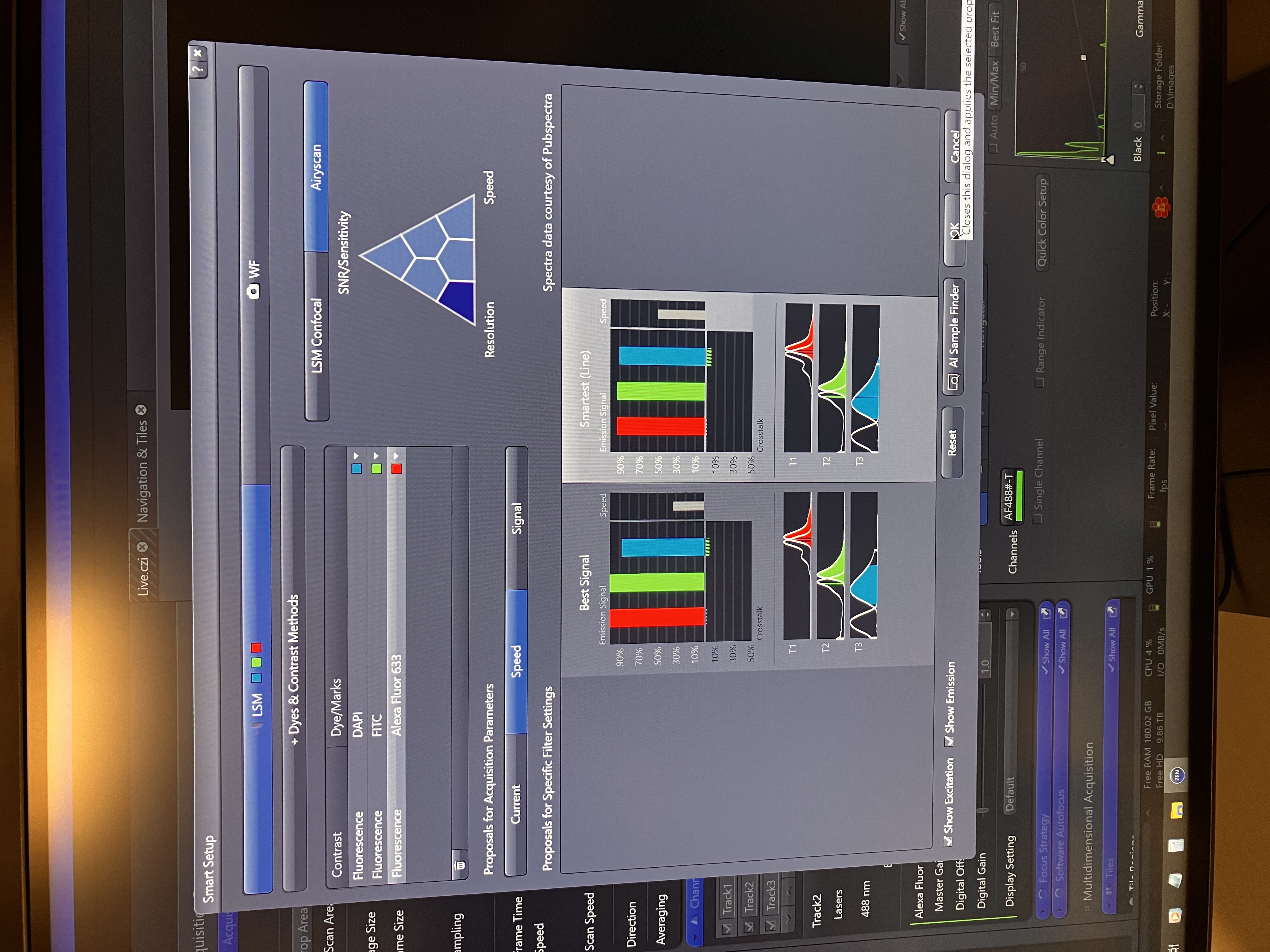
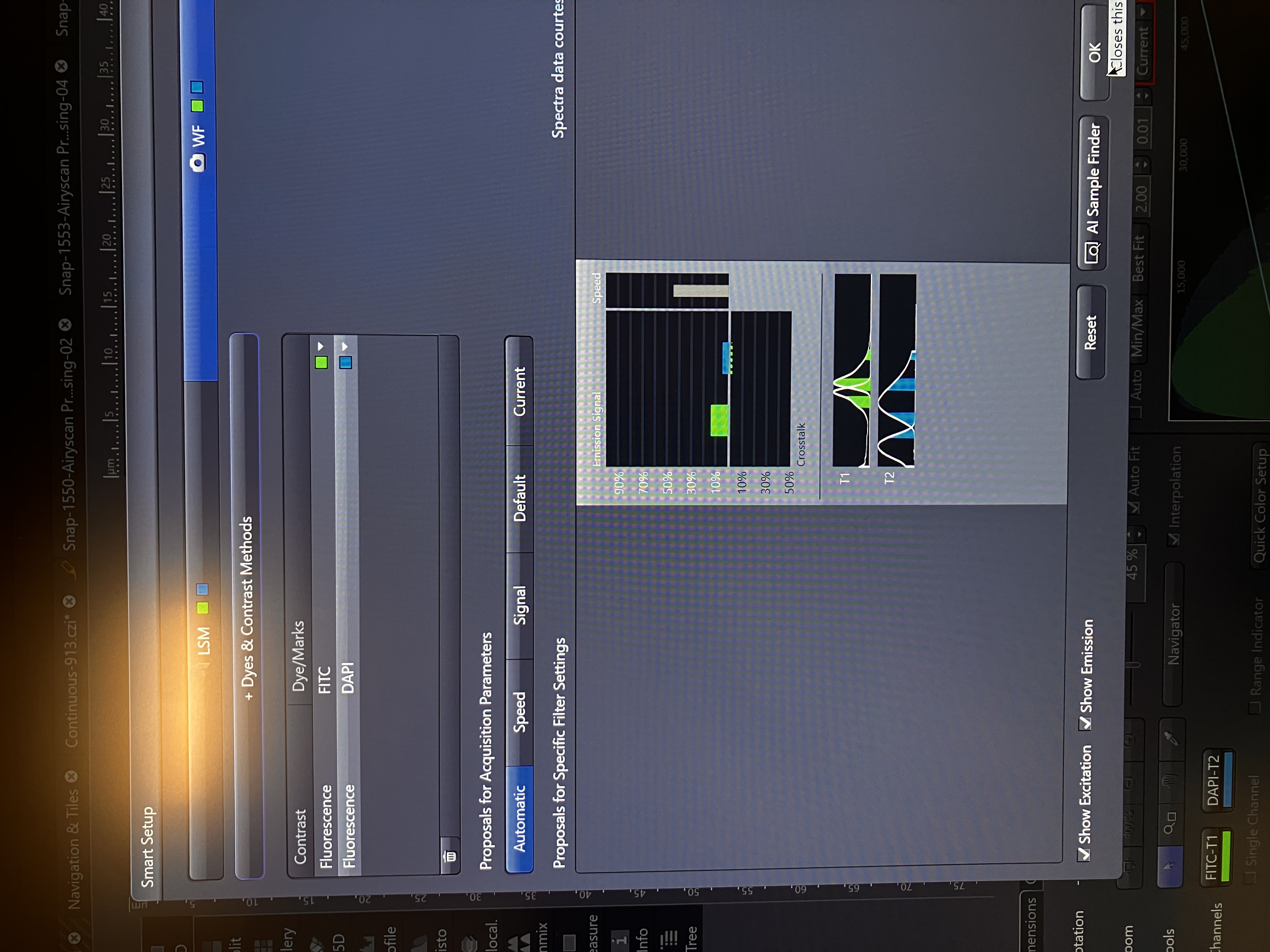
3.1.1.1 Using Smart Setup
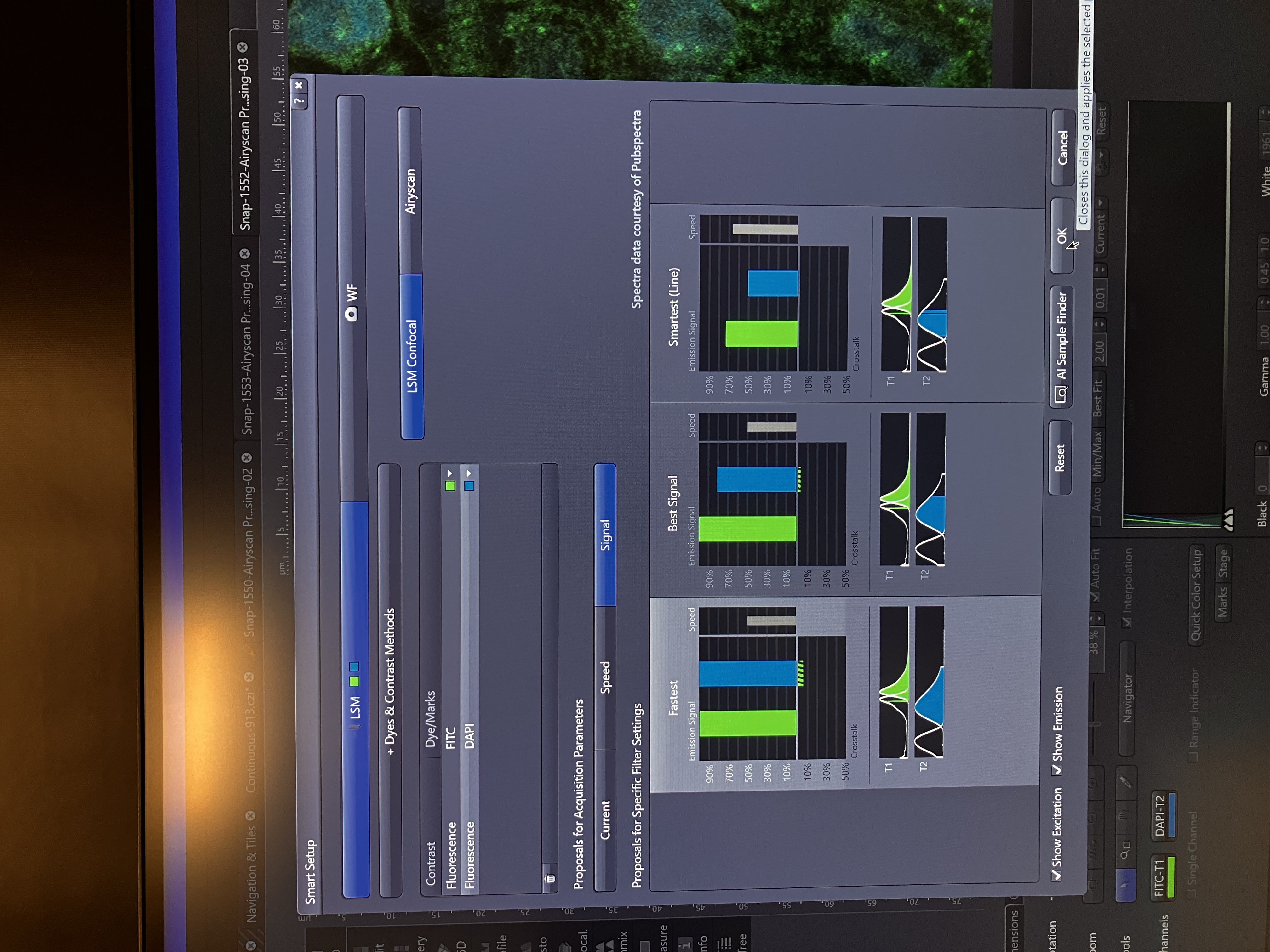
- Make sure “LSM” is selected.
- Add the fluors you want to image by clicking “+ Dyes & Contrast Methods” and then selecting from the available options. Note that you search for fluors that are not showing up by default.
- Select “Airyscan” and then click the bottom left corner of the triangle (next to “Resolution”).
- Choose the proposal that best suits your needs.
- Click “OK” to finish.
3.1.1.2 Loading a Past Setup
- At the top of the screen on the left side, under “Locate” and “Acquisition,” you can find the name of the current setup. Click on it and toggle to the setup that you would like to load.
3.1.1.3 Manual Setup
- Go to “Imaging Setup” on the left side of your screen. If there are tracks there, you can either delete them or alter them.
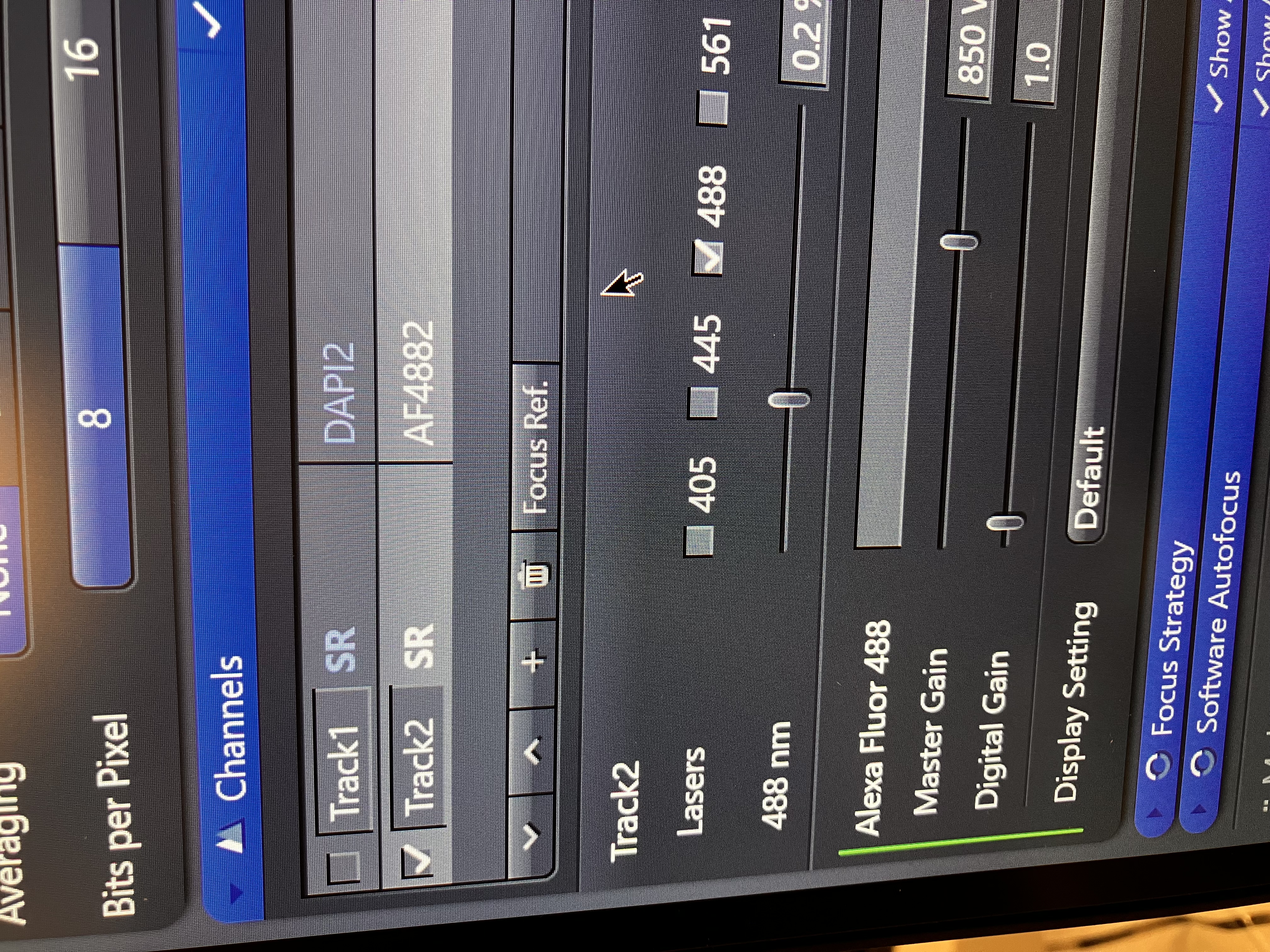
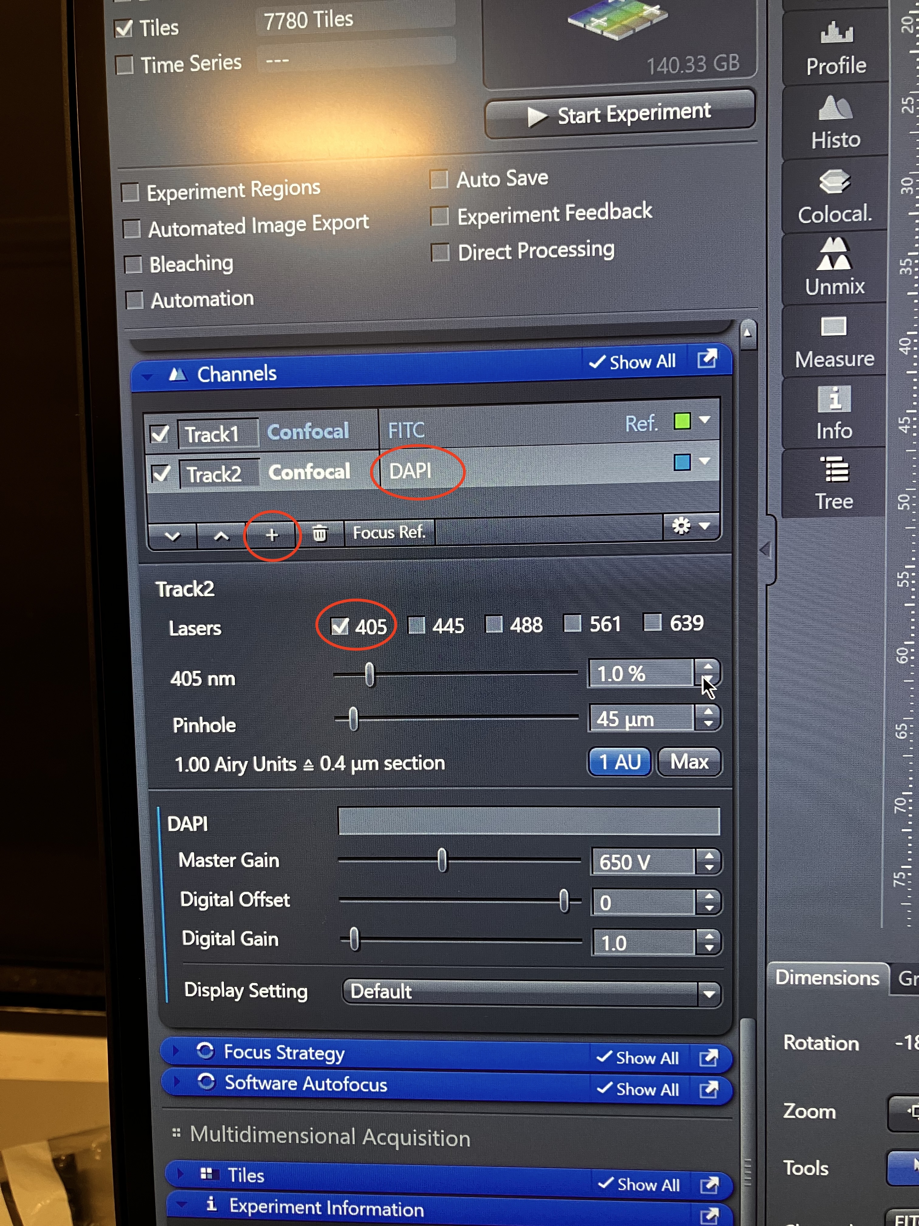
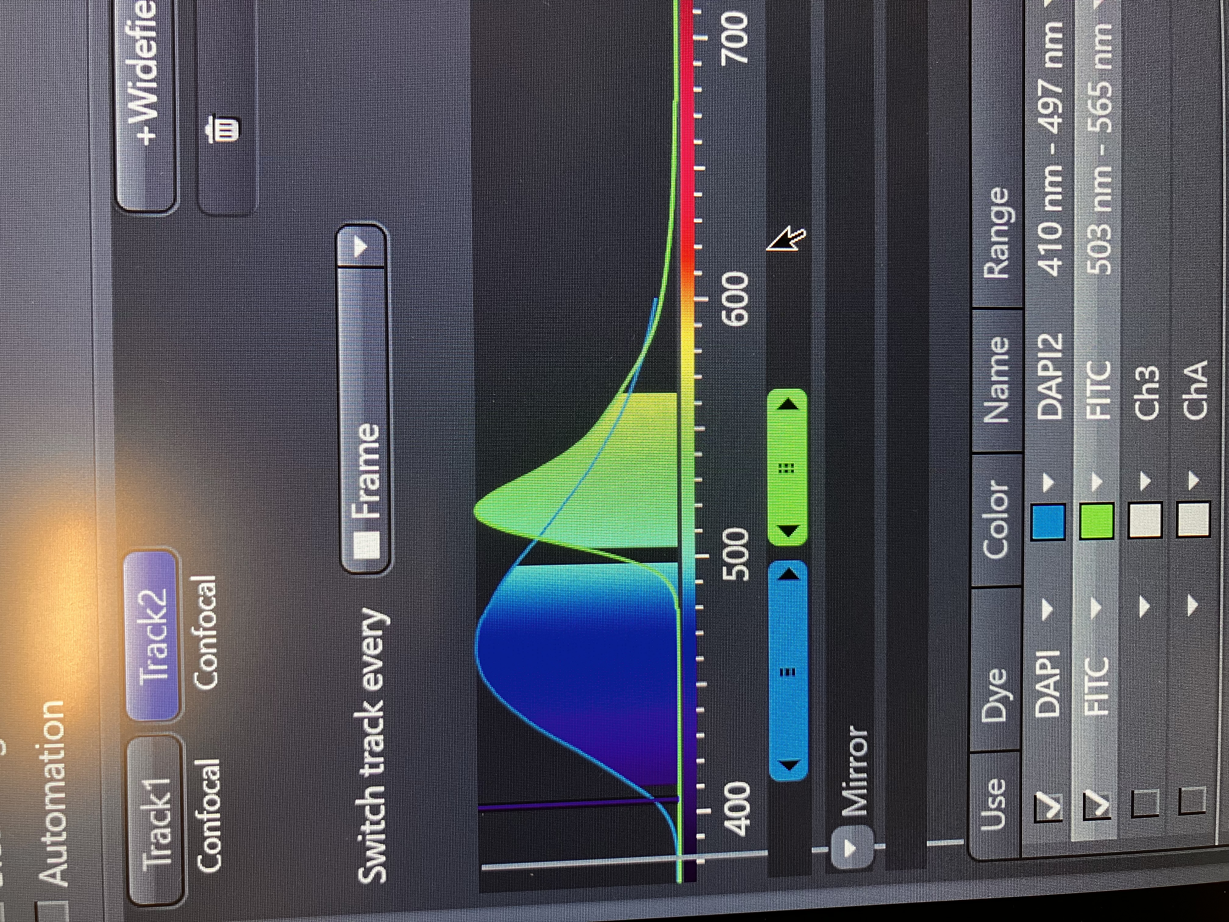
- Add the specific tracks you want, specify the dye for each (top), and check the corresponding laser for each (bottom):
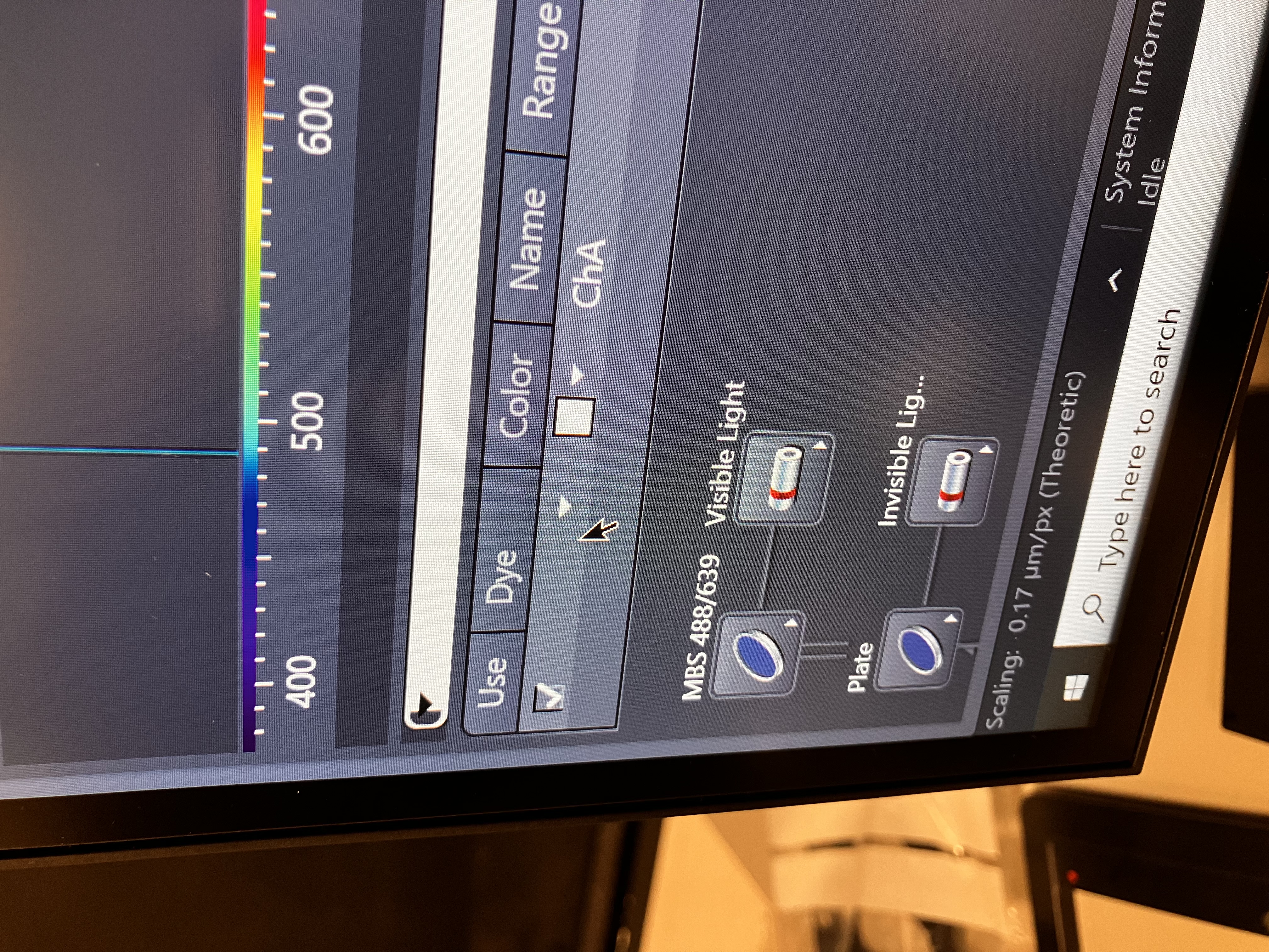
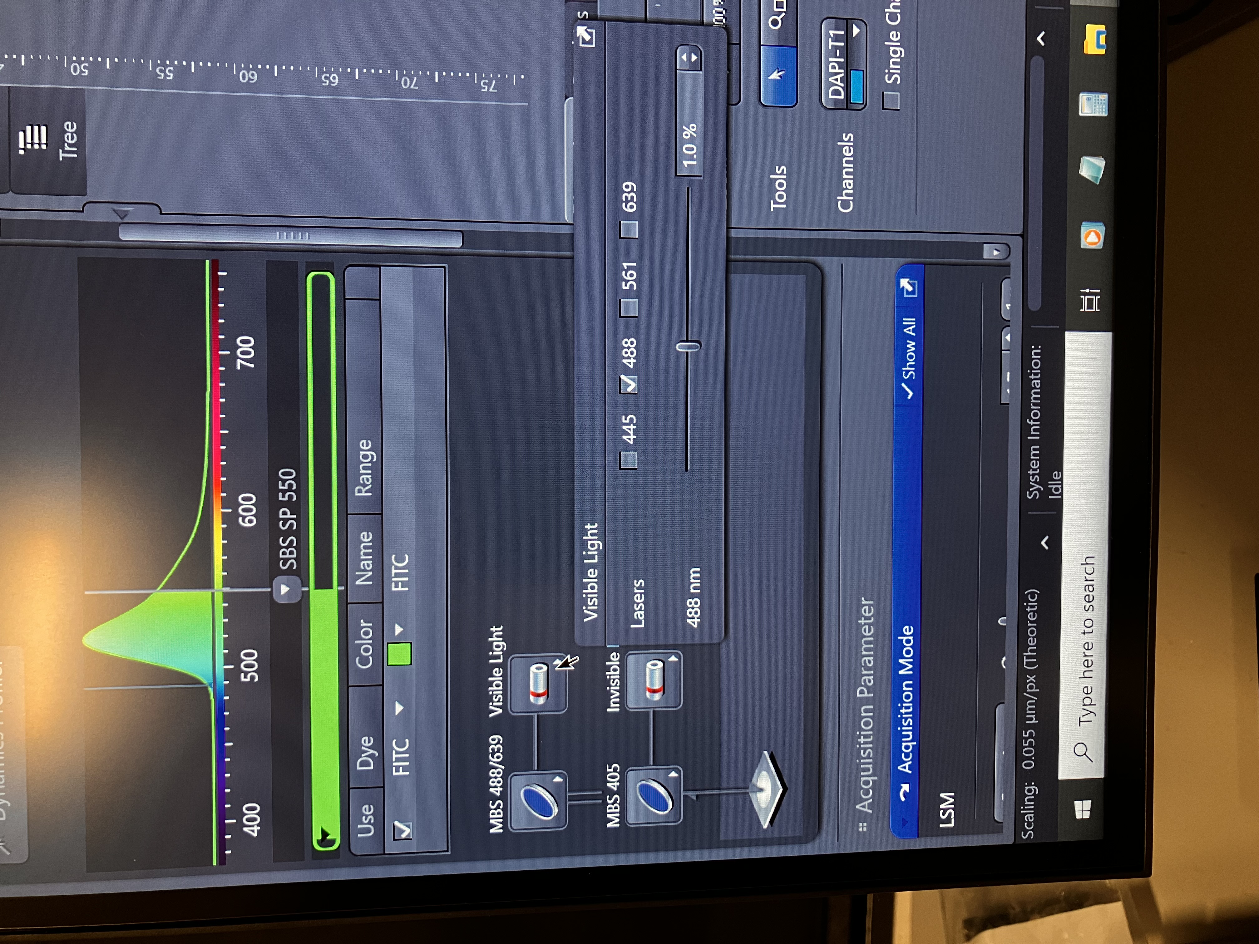
- Adjust the filters for each:
- Note here that there are two separate laser paths: one for visible light and one for invisible light. Each of these paths employs its own beamsplitter, which you can customize by clicking the icon to the left of the laser icon.
3.1.1.4 Adjusting Your Acquisition Scheme:
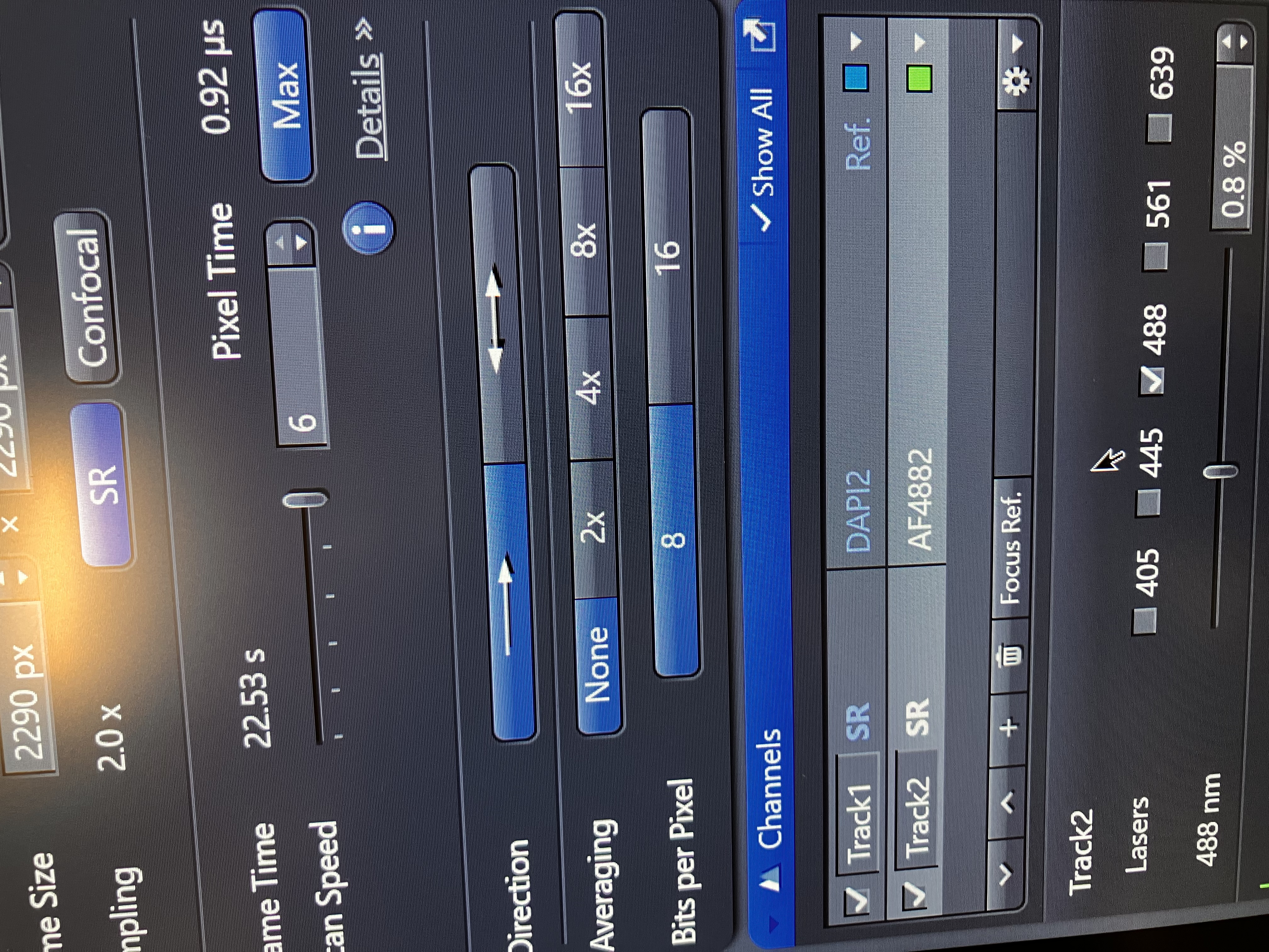
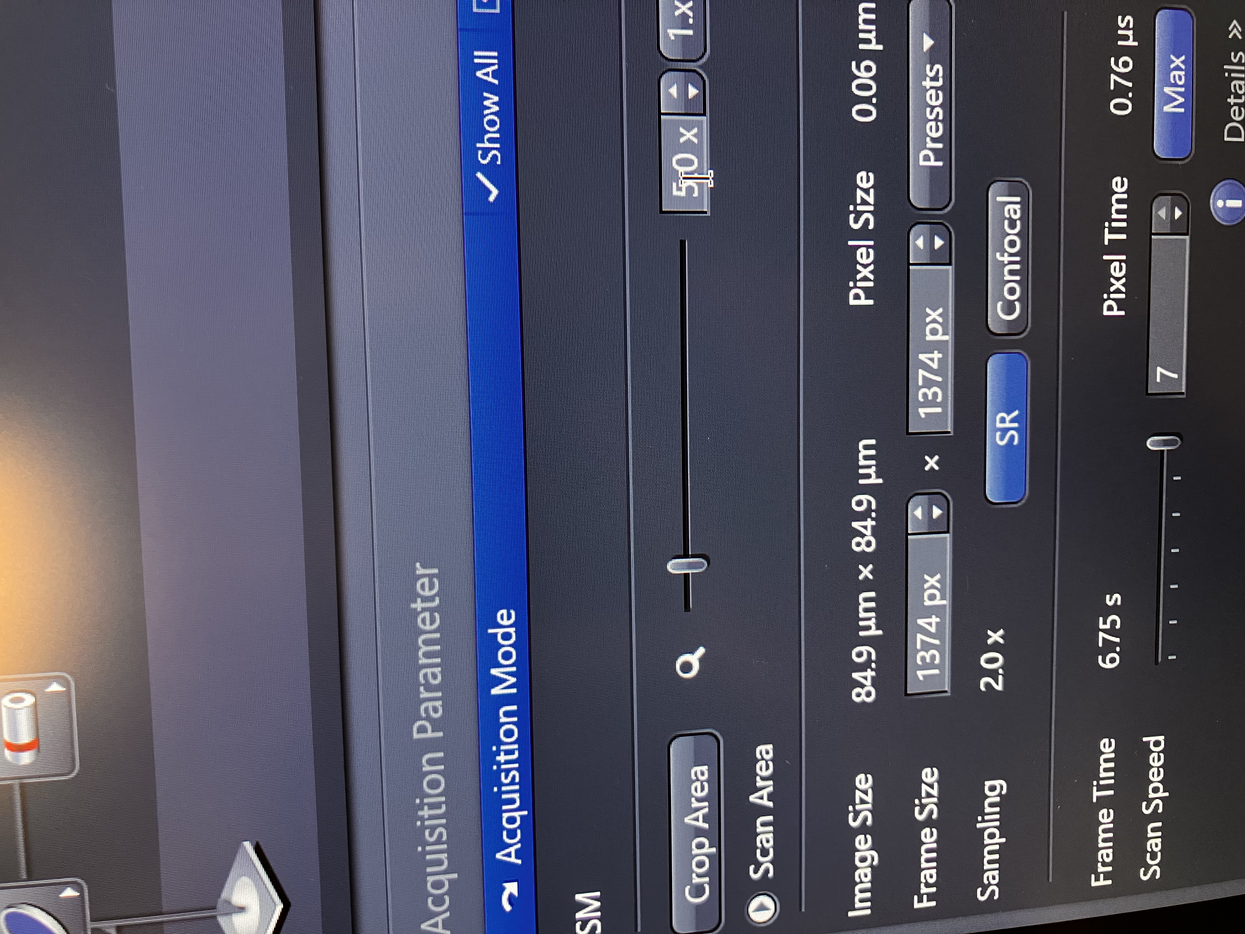
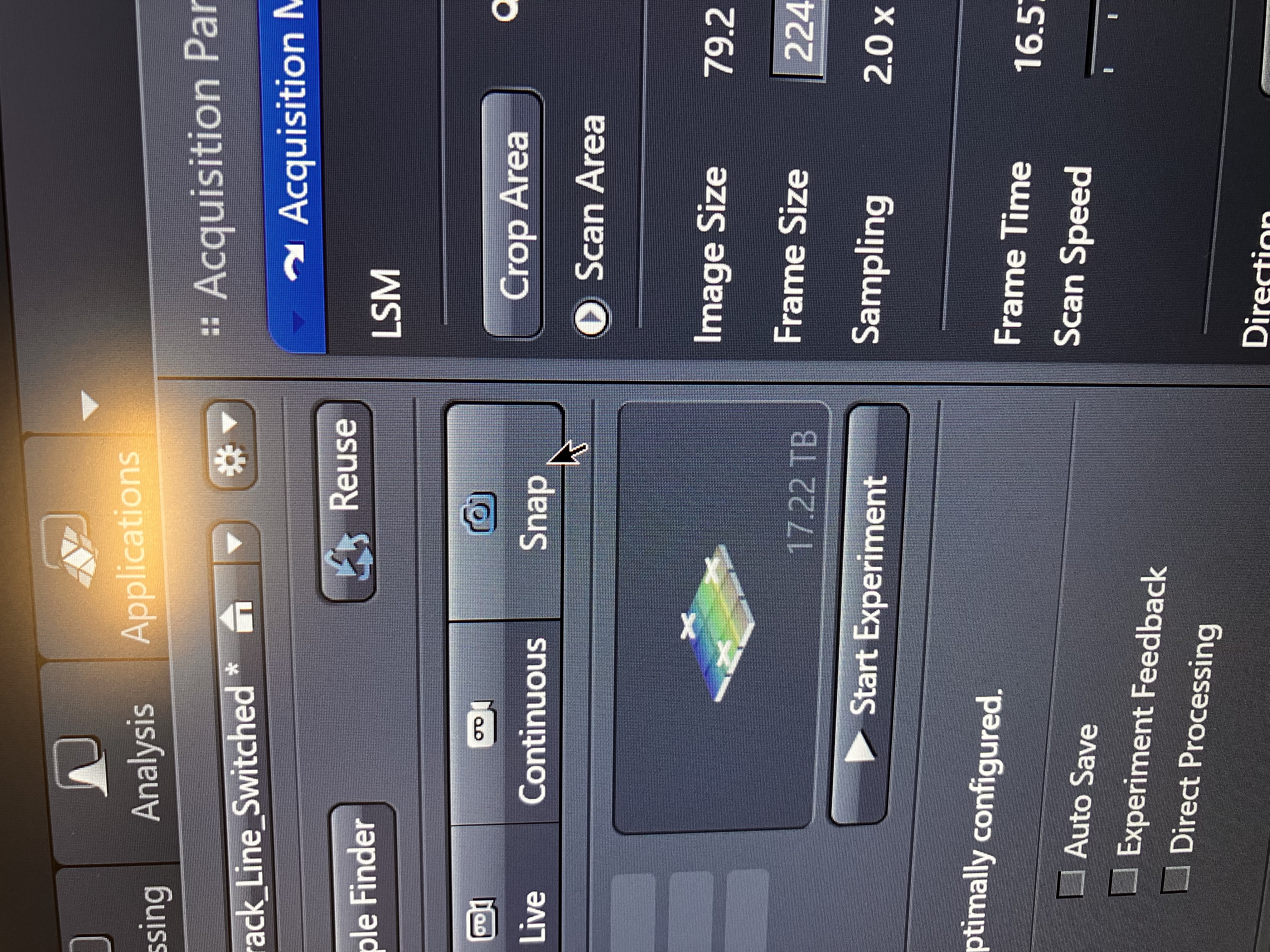
- Shown below are some settings to pay attention to in the acquisition part:
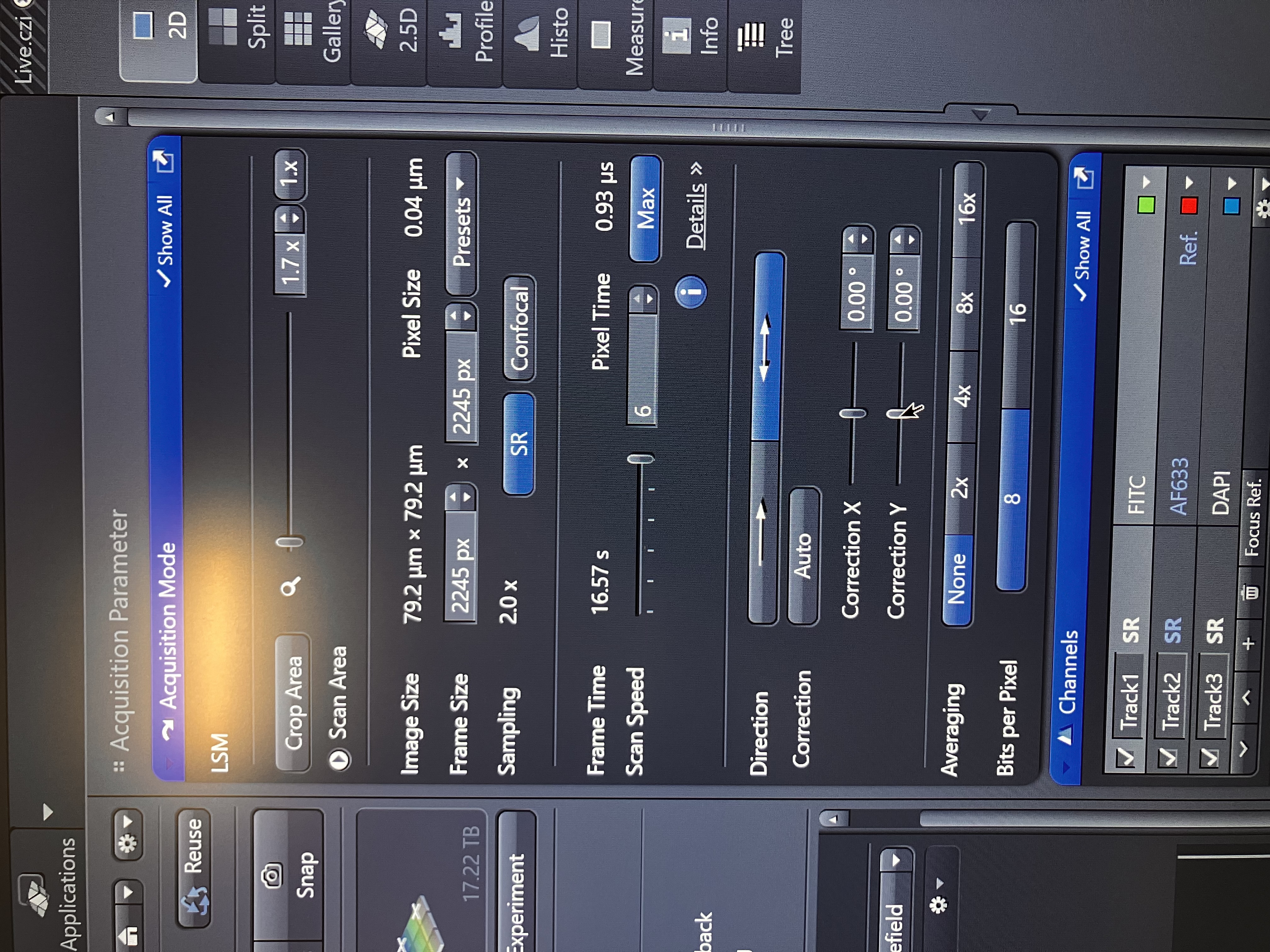
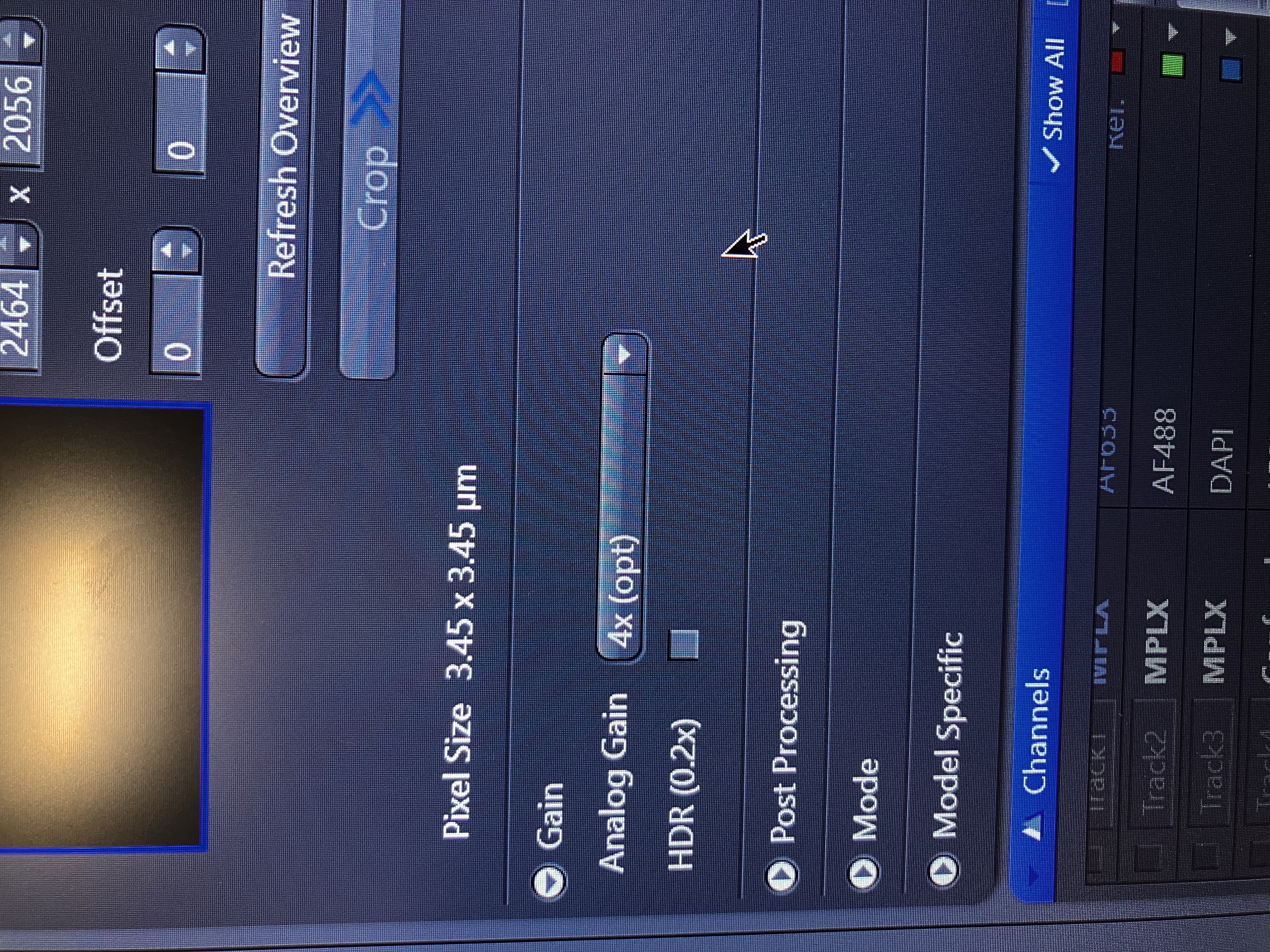
- Crop area refers to the field of view. By default, it is set to 1.7x. However, you can increase this number to crop the field of view. Frame size refers to the number of pixels that will comprise the image. In “Live” mode, this is set to 512 x 512. “Continuous” mode uses the parameter that you set here. The “SR” button will ensure that your sampling is adequate for SR-level resolution.
- Shown below are some settings to pay attention to in the channel part:
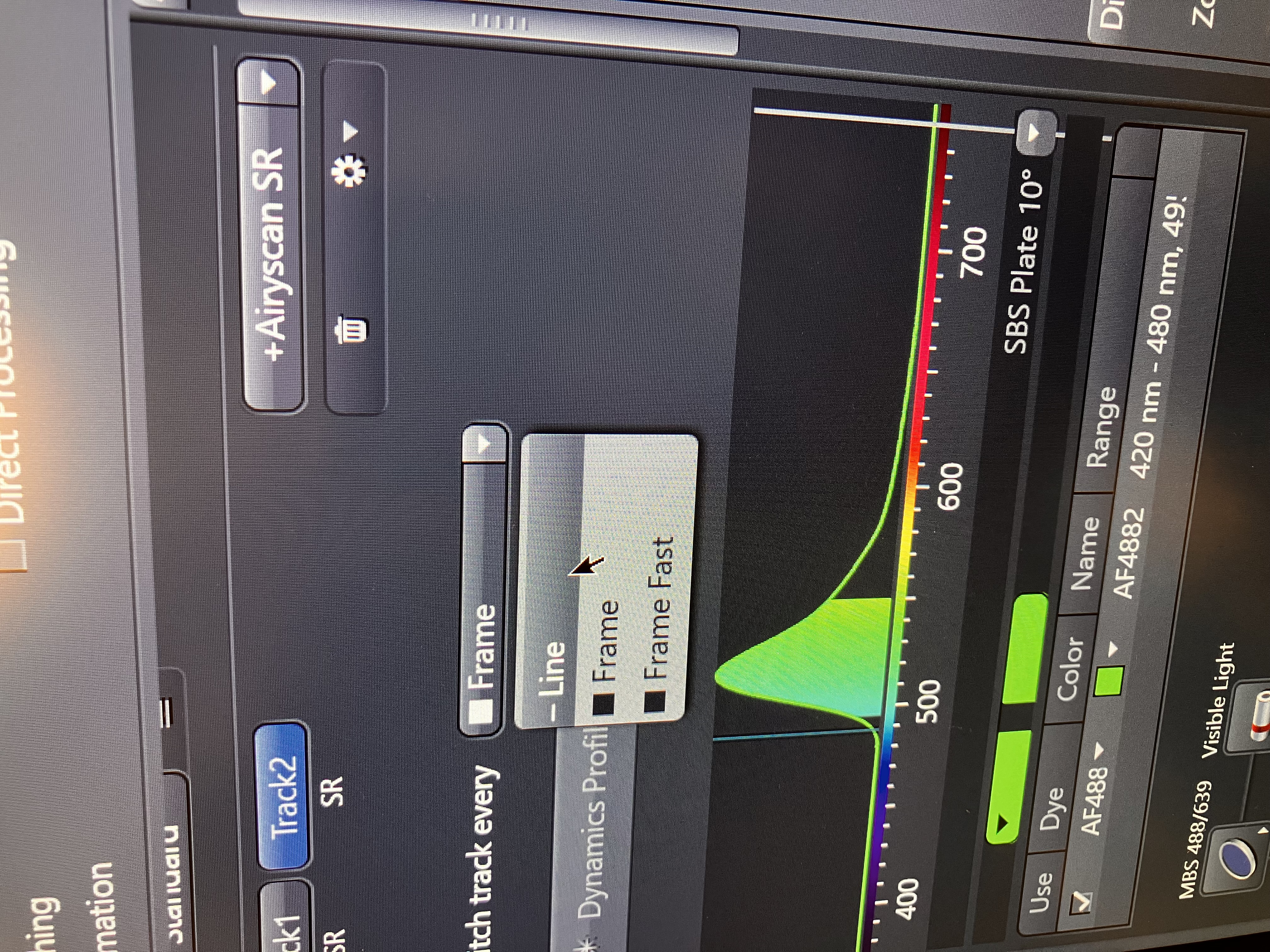
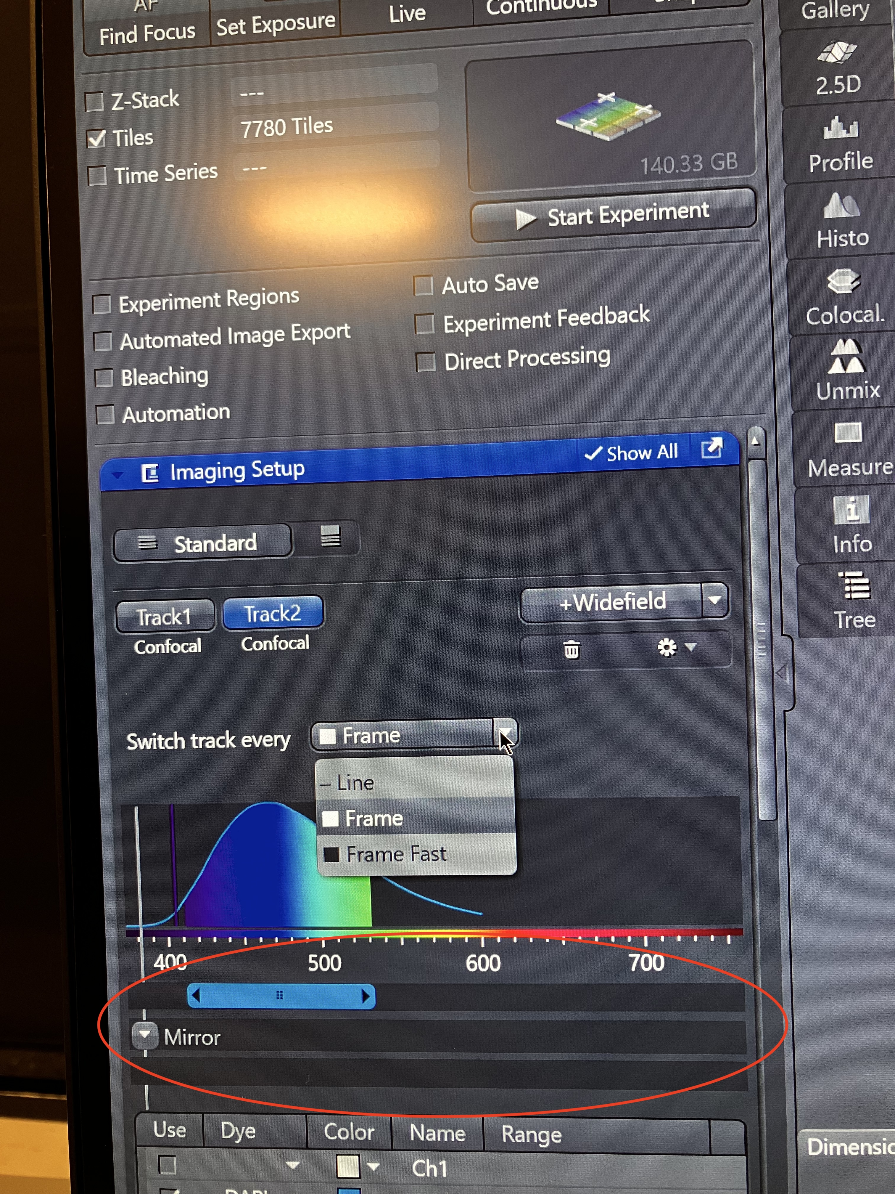
- Frame means that the entire frame will be scanned and imaged for each track in a sequence. Line means that each line of the frame will be imaged for each track in a sequence.
- Remember that each time the track changes, the laser and/or the filters must switch inside of the machine (unless no changes are necessary). So, if you have tracks with different filters and different lasers, if you use line mode, then many switches must occur at the end of each line of the frame. For a large frame, this can be time consuming.
- Balance your acquisition scheme to achieve quality imaging in a reasonable amount of time (i.e. without much switching). This does not always mean that frame is the best choice because there are usually fewer switches. If you can keep the filters the same for each track, and if you are not dealing with excitation bleed through (see Imaging Considerations), then line is often the better choice.
3.1.2 Ensure You Can See Something & Get in Focus
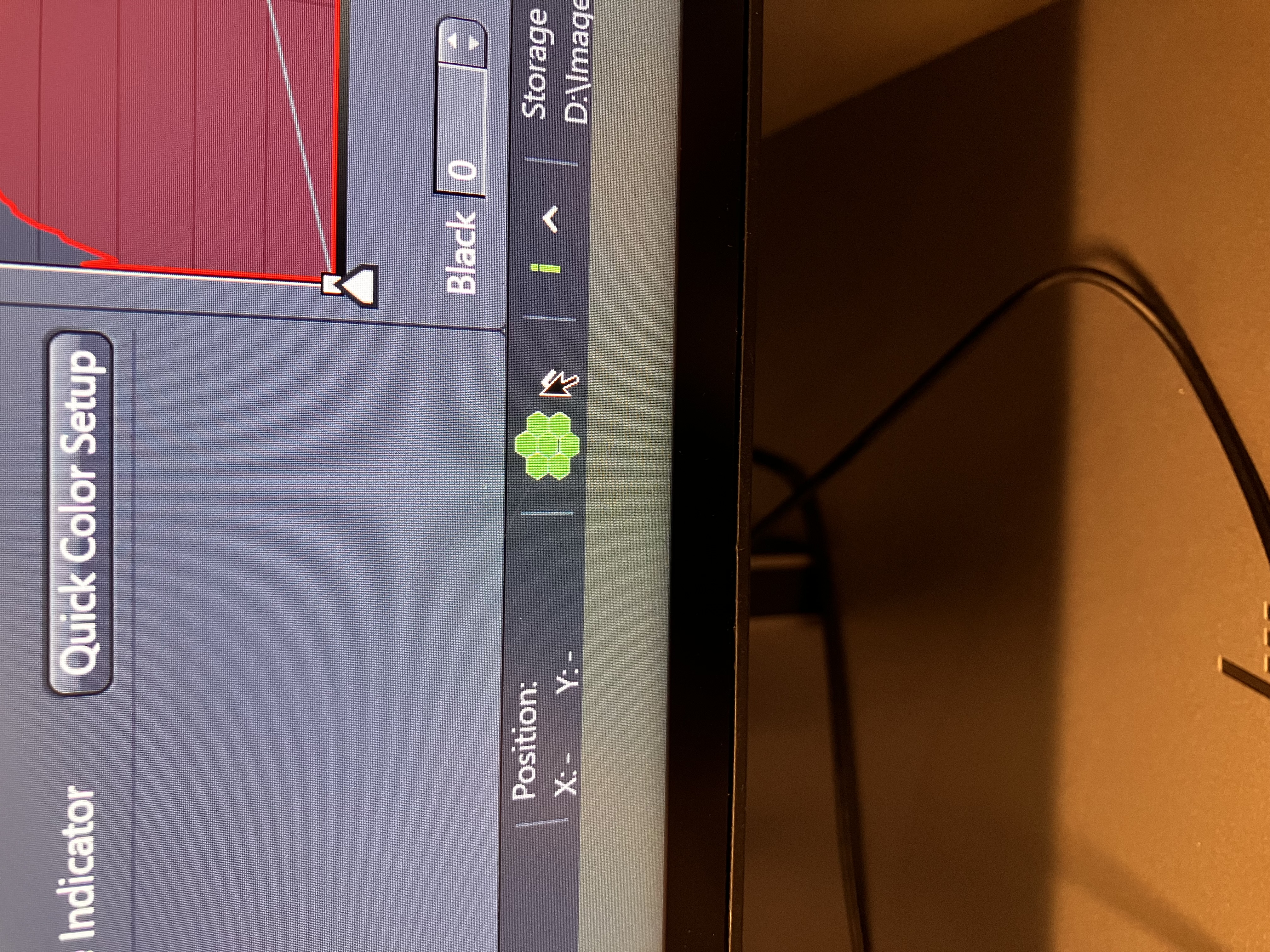
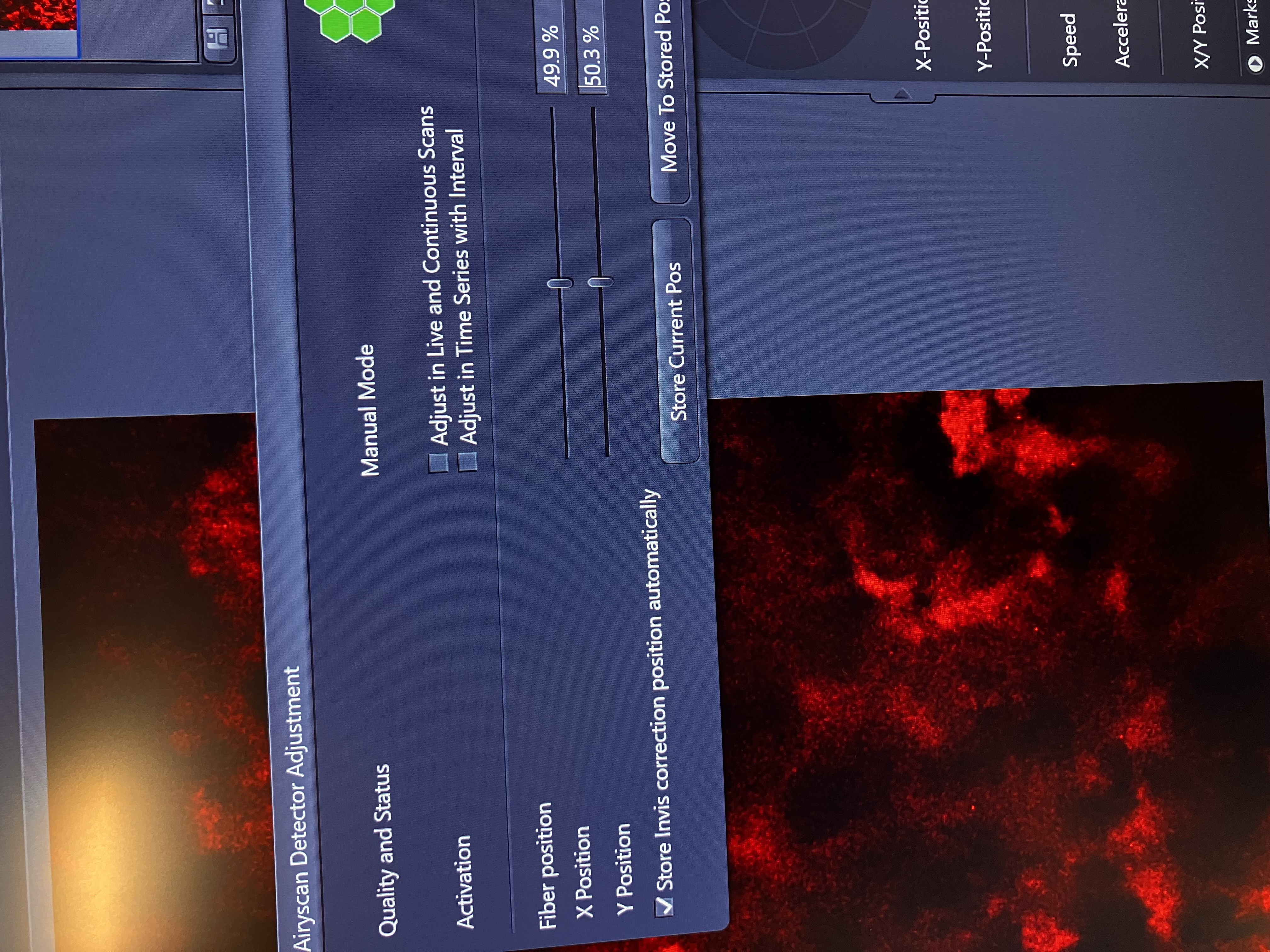
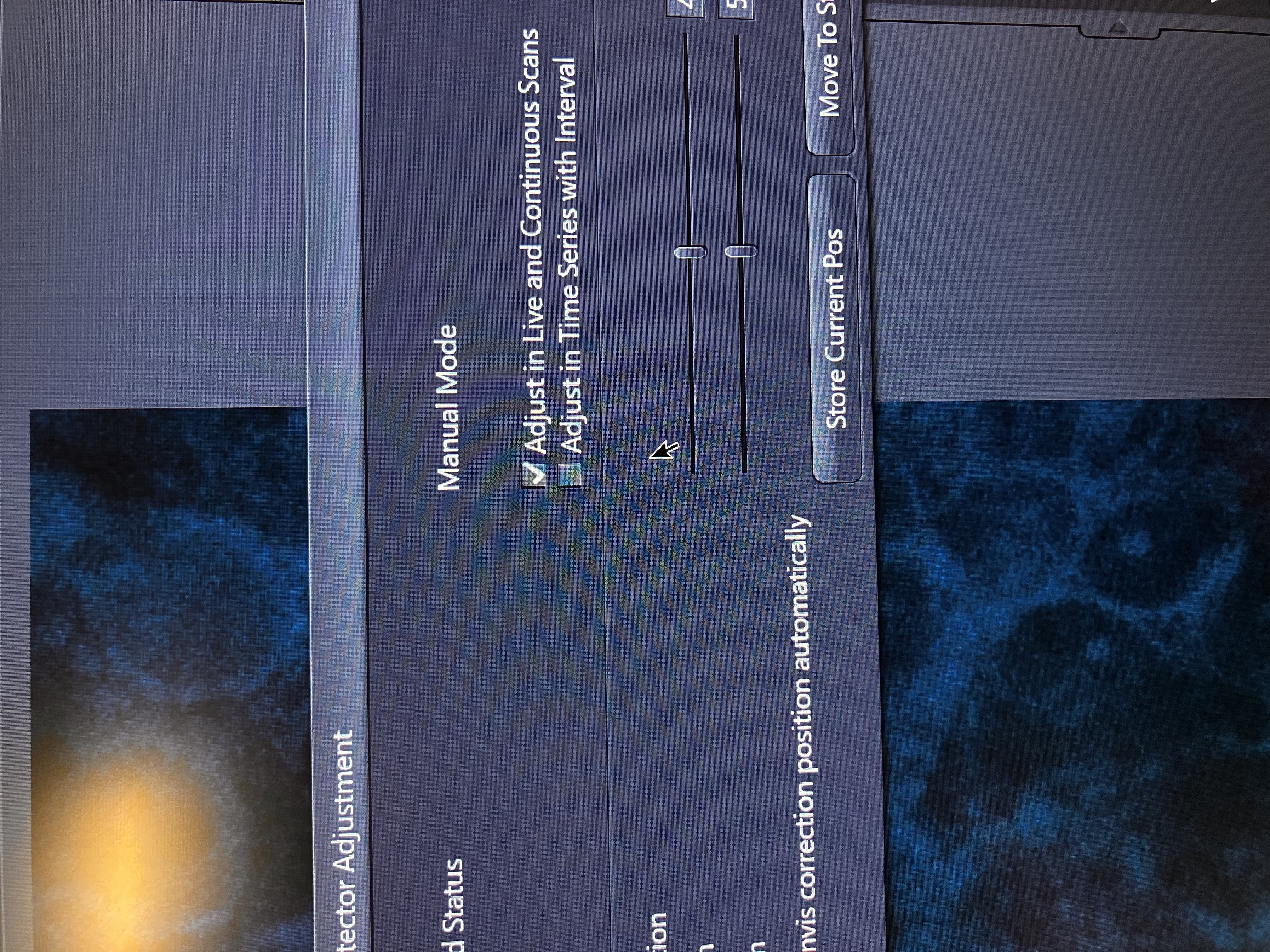
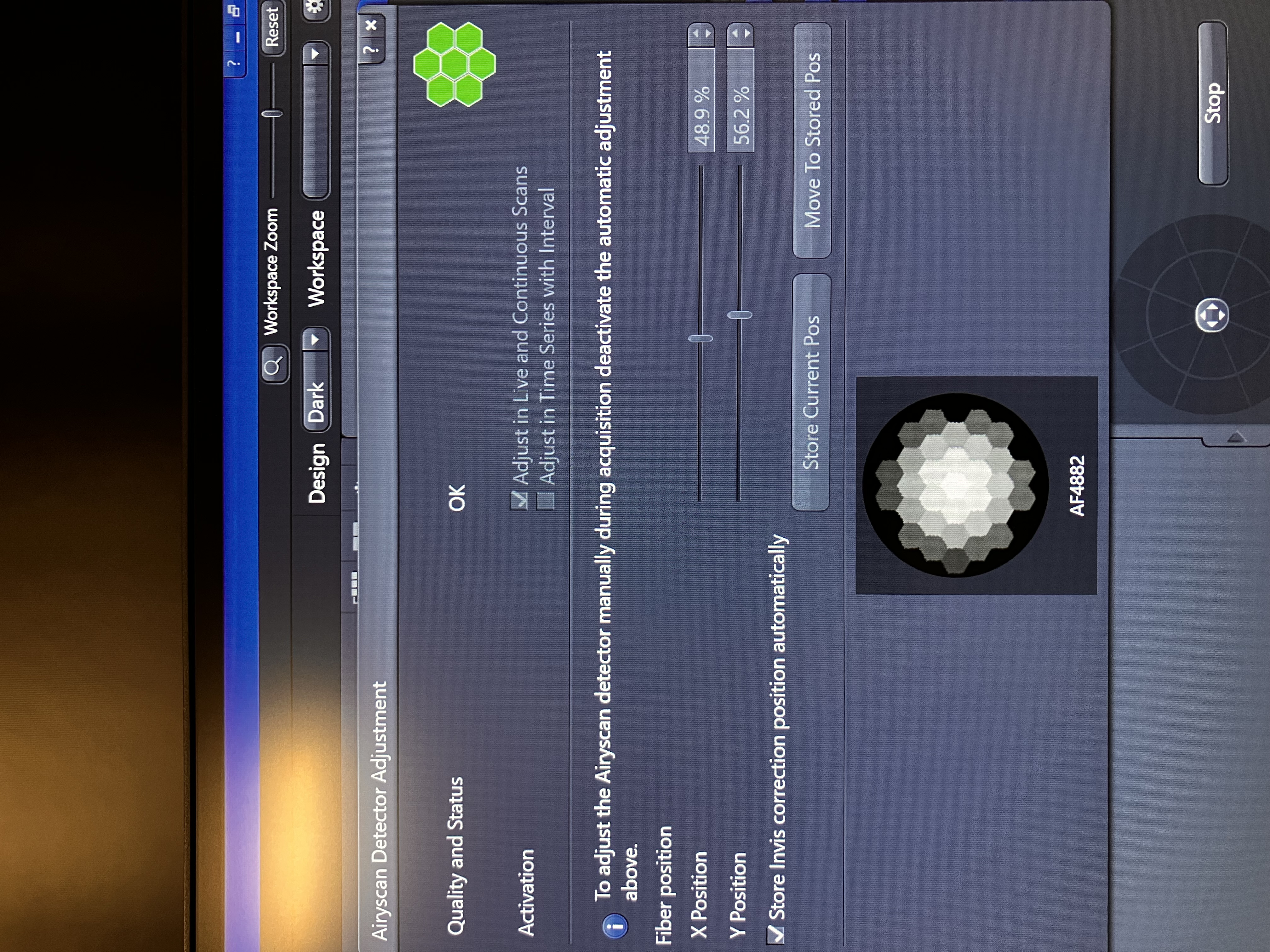
- Ensure that the Airyscan alignment sliders are at ~50% and that Airyscan alignment is not adjusting automatically. Click the honeycomb icon at the bottom of the screen and then adjust the settings to be like the following:
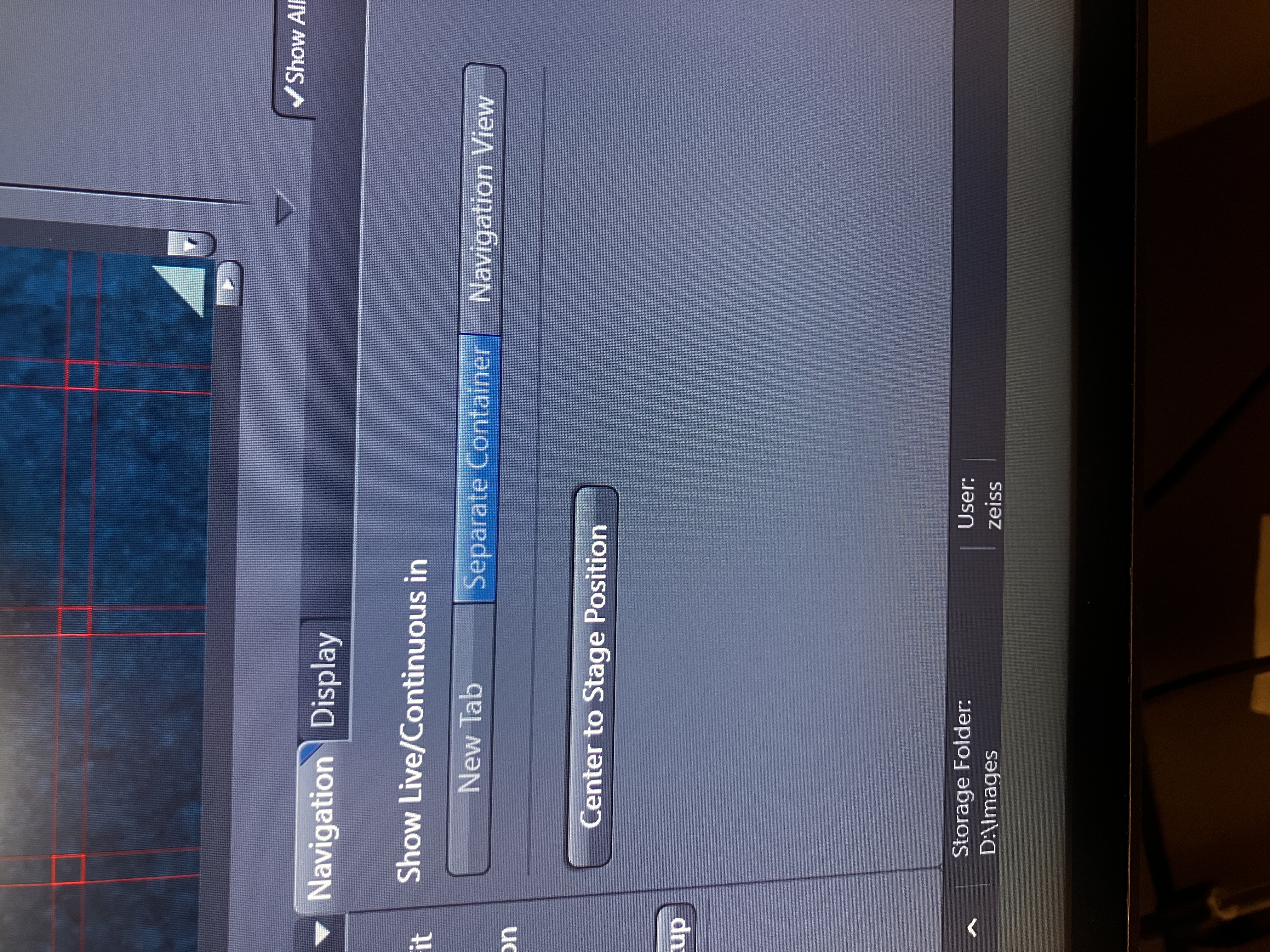
- Ensure that the stage is at the position that you saved during the setup procedure by tapping “Pos. 2” on the touch pad. It can be helpful to select the following setting to keep the navigation view present:
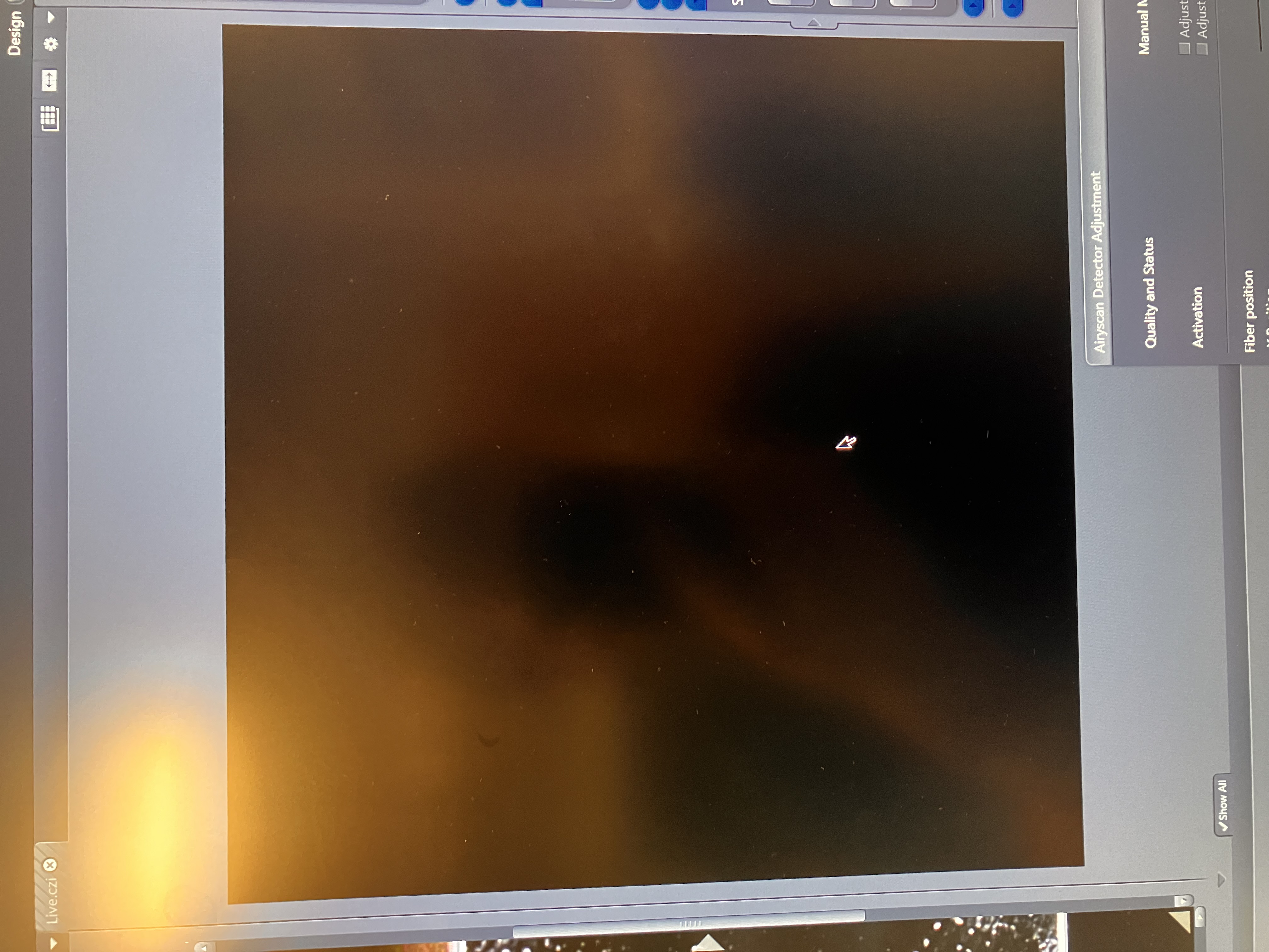
- Select a track and then click “Live.” You should see at least some signal.
| The optical system has slightly changed because you changed detectors when you selected Airyscan. So, the focus is off by a small amount.
- Scan up and down with the fine focus knob or with the computer by slowly scrolling with the mouse while holding the “control” key.
- Stop scanning where the signal is brightest. Note that the focal plane is very thin. You could be only a fraction of a full mouse scroll between this (top) and this (bottom):
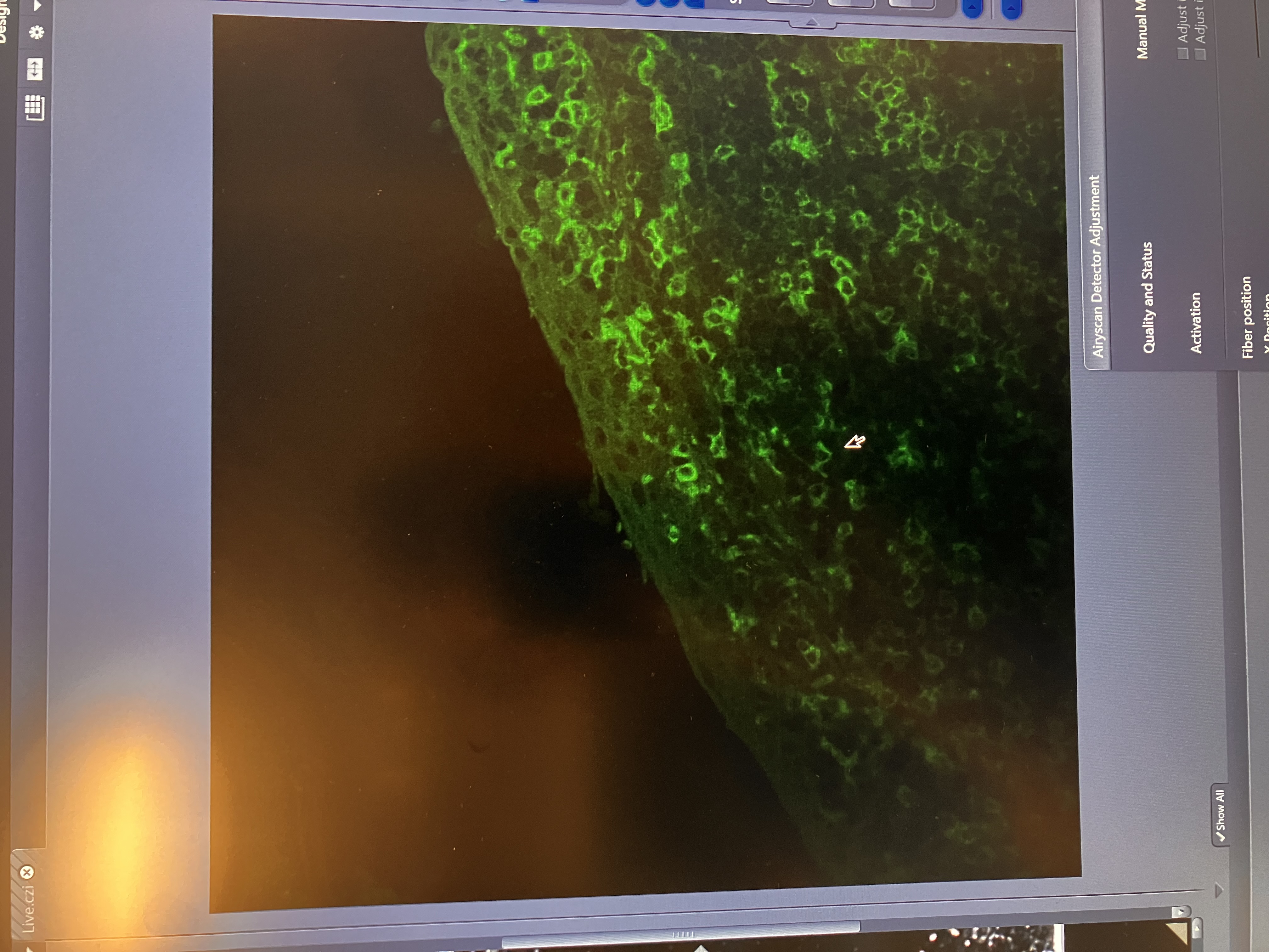 | Now, you are in focus in this new optical system with the Airyscan detector.
3.1.3 Toggle through the Tracks and Optimize View Settings
- For Airyscan, laser power should be in the range of near 0 to ~1.5.
- Master gain should be in the range of 600 to 900. Digital gain should typically stay set to 1.
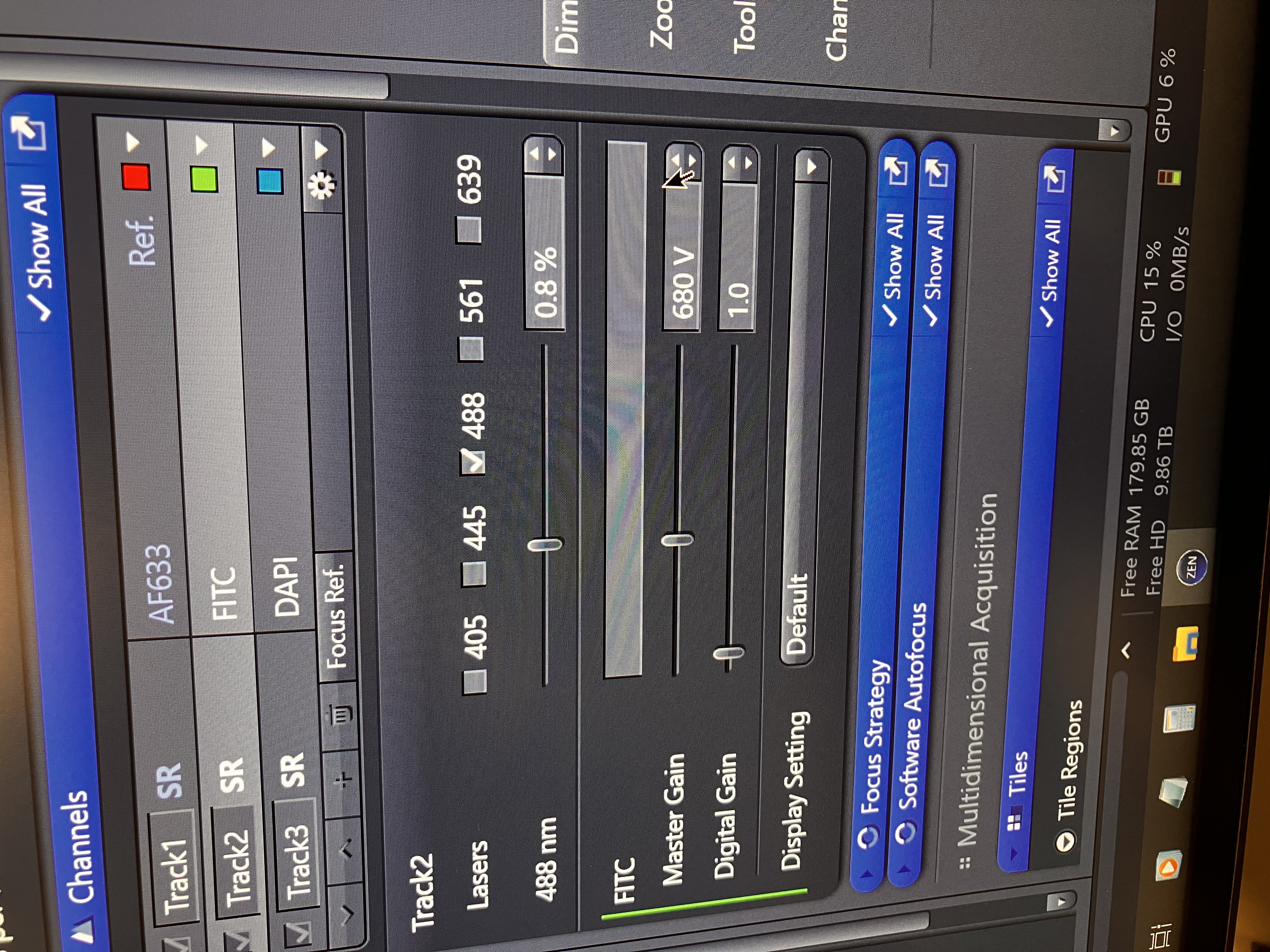
Increasing gain will increase the noise of the image. Increasing laser power can cause photo bleaching. Essentially, you want to increase the laser power as much as you know you can without photo bleaching, then adjust the gain accordingly.
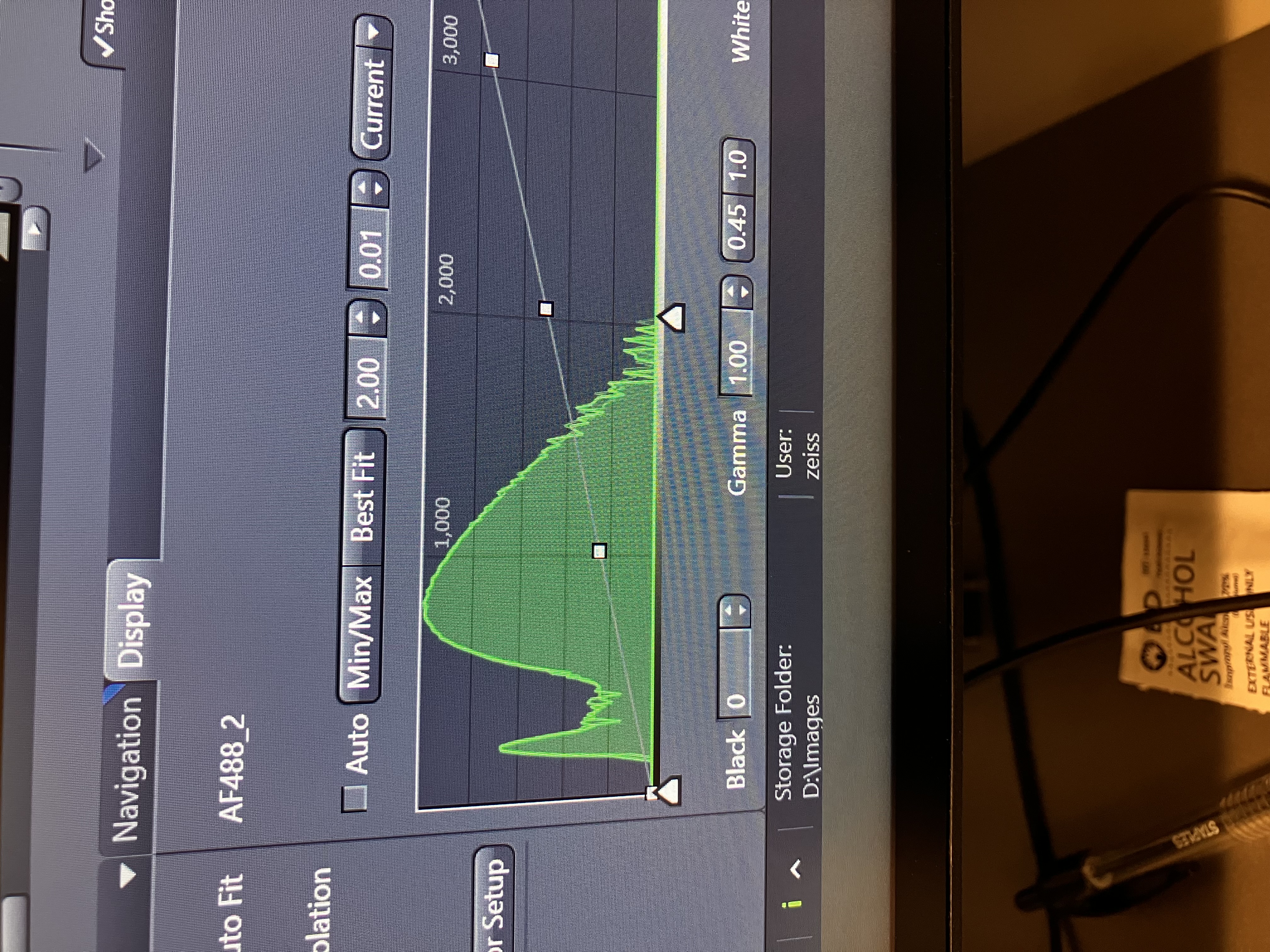
- Ensure that the histogram for each track is left skewed and has a range that fills about half of the dynamic range. Do not worry about how the image looks yet.
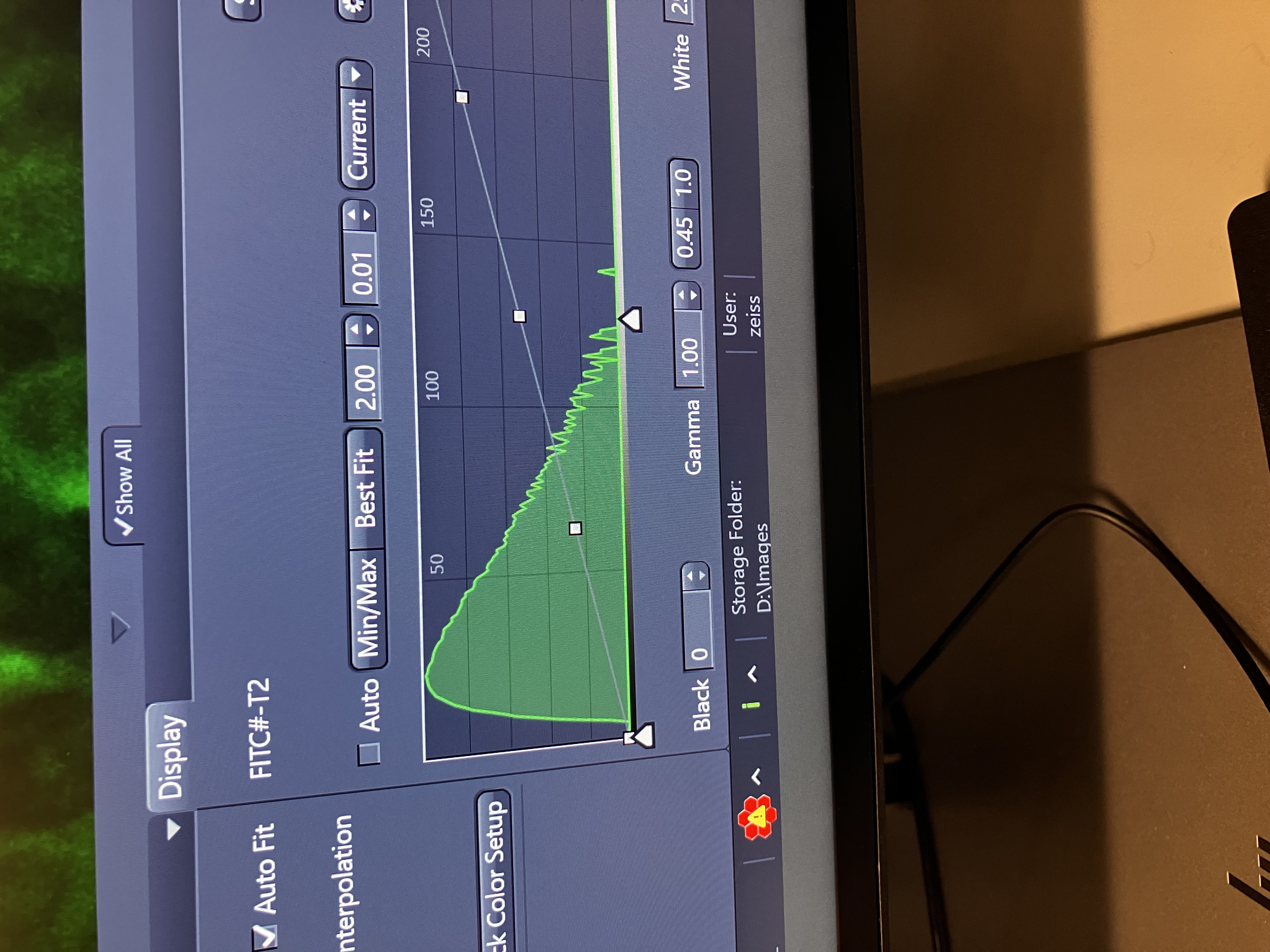
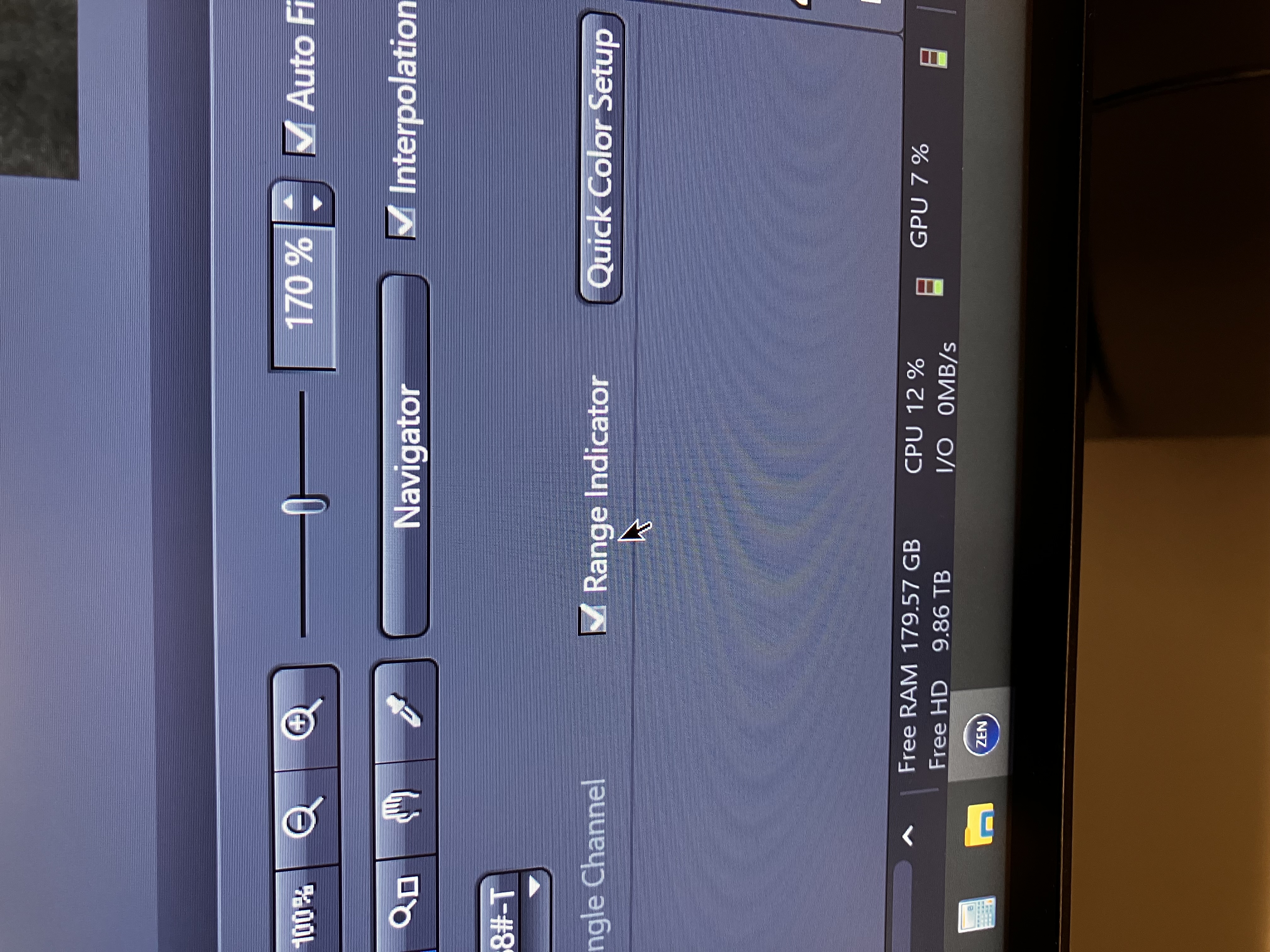
- Check the range indicator for any saturated pixels. There should be no saturated pixels at all. Saturated pixels display as red. Having saturated pixels can negatively affect deconvolution methods in processing steps downstream.
- Using “Line” instead of “Frame” will keep the master gain setting the same for all tracks. So, if you switch between tracks and change the master gain between them, the previous gain settings will be overwritten.
3.1.4 Airyscan Detector Alignment
- Start with alignment for tracks that will capture visible light. Check only one of the visible tracks (the Core recommends you check the track capturing green light).
- Open the Airyscan alignment settings again and allow automatic adjustments.
- Start “Live” and let the alignment run. You will notice that the histogram will change a bit. If no pixels are saturated, it is okay.
- When alignment is okay, turn “Live” off.
- Next, align tracks that will capture UV (invisible) light.
- Keep the one visible track checked, and now check the UV (invisible) light track.
- Important Note: Tracks that measure DAPI are set to be UV (invisible) light tracks, by default, if you used Smart Setup.
- If using frame, adjust the crop size to ~5x or higher and/or make the frame size smaller than the highest option (this will save time).
- Start “Continuous” (next to “Live”) and let the alignment run.
- Stop “Continuous” when alignment is okay for both selected channels.
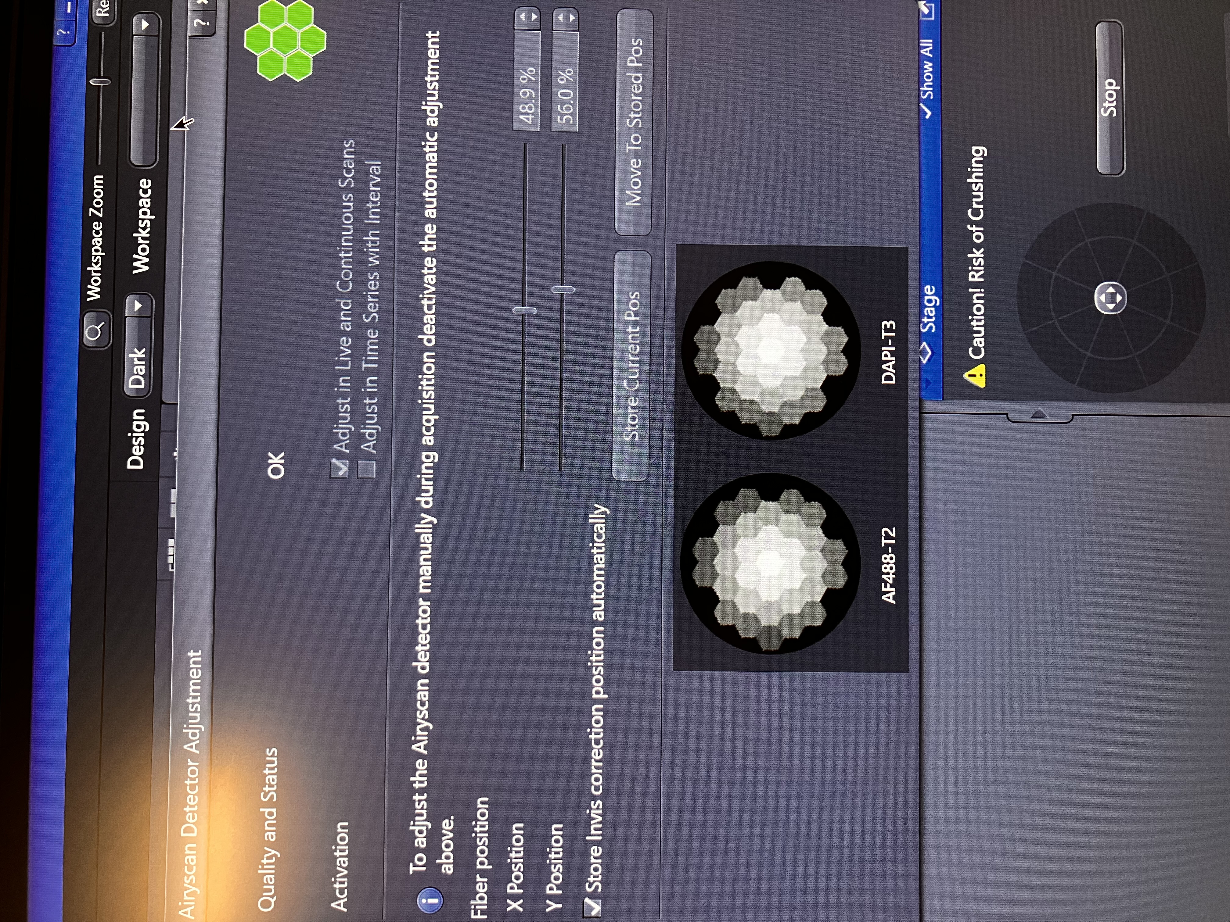
- Again, ensure no pixels are saturated after the histogram changed a bit.
- Important Note: This can take a while due to switching between tracks. A good way to speed this up is to keep the acquisition settings similar or identical across the tracks. The beam splitter setup being different across the tracks can often cause slow switching.
- Turn off automatic adjusting of the Airyscan alignment by unchecking the box in the figure above.
3.1.5 Capture an Image and the Associated Data
- Change the crop size back to what you desire.
- Click “Snap” next to the “Continuous” button.
- Let the software run.
- Note that you may choose to implement averaging.
3.1.6 Perform Airyscan Processing to Acquire a Final Flat Image
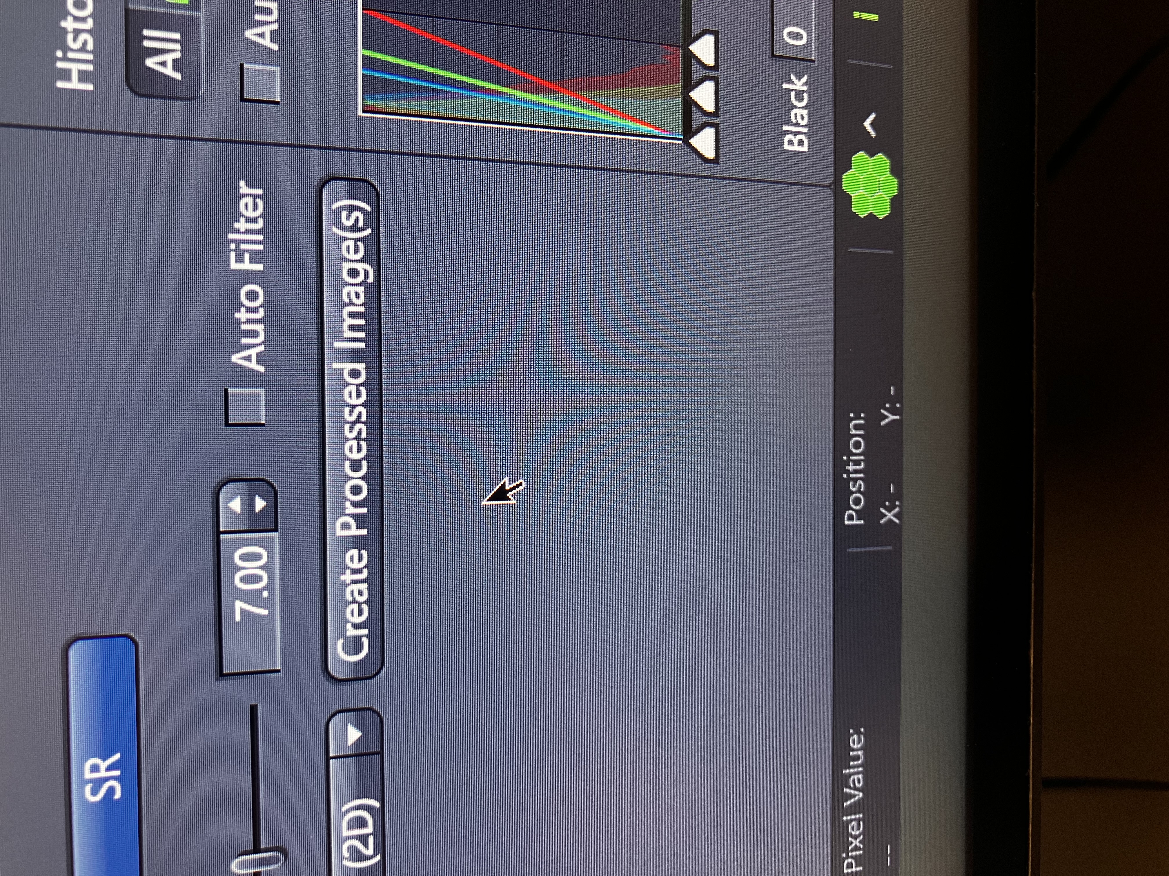
- At the bottom of the screen, select the “Airyscan” tab.
- Adjust the parameter as you wish. Typically, adding between 0 and 0.5 to the default value works best.
- Finally, click “Create Processed Image.”
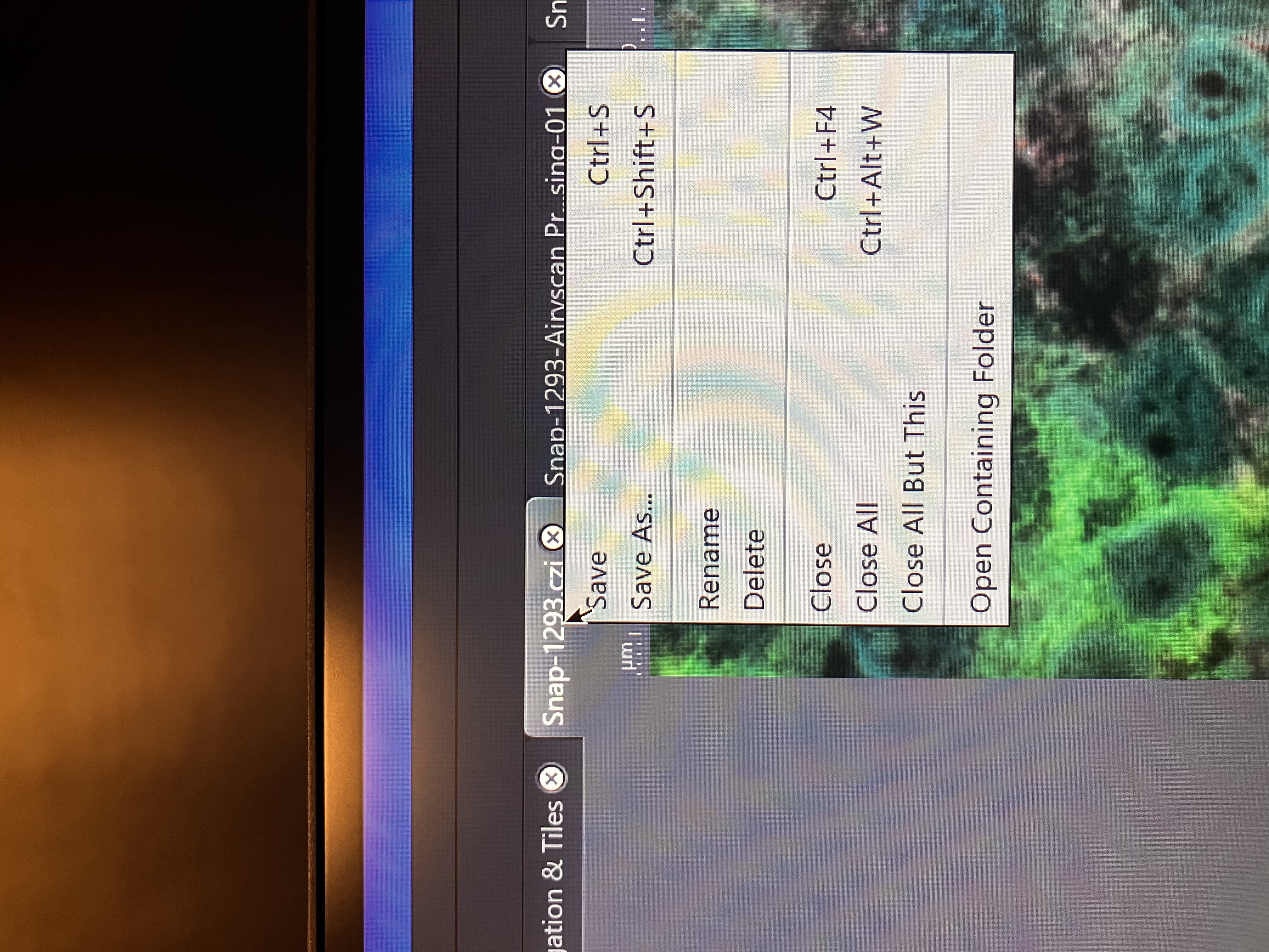
- Save the image and/or the raw data by right clicking on the file’s name:
3.2 Confocal Mode
The following outline of steps should get any user a single image acquisition using the confocal (without Airyscan) modality of this microscope.
When confocal mode is used, simultaneous acquisition is possible. This means that light from multiple channels can be imaged on the same track at the same time. Using this feature can speed up imaging, but it can lower image quality, since there is the possibility that light is assigned to the “wrong” channels.
3.2.1 Set Up Tracks and Acquisition Scheme
You can use Smart Setup, load a past setup, or you can do this step manually.
3.2.1.1 Using Smart Setup
- Make sure “LSM” is selected.
- Add the fluors you want to image by clicking “+ Dyes & Contrast Methods” and then selecting from the available options. Note that you search for fluors that are not showing up by default.
- Select “LSM Confocal.”
- Choose the proposal that best suits your needs.
- Click “OK” to finish.
3.2.1.2 Loading a Past Setup
- At the top of the screen on the left side, under “Locate” and “Acquisition,” you can find the name of the current setup. Click on it and toggle to the setup that you would like to load.
3.2.1.3 Manual Setup
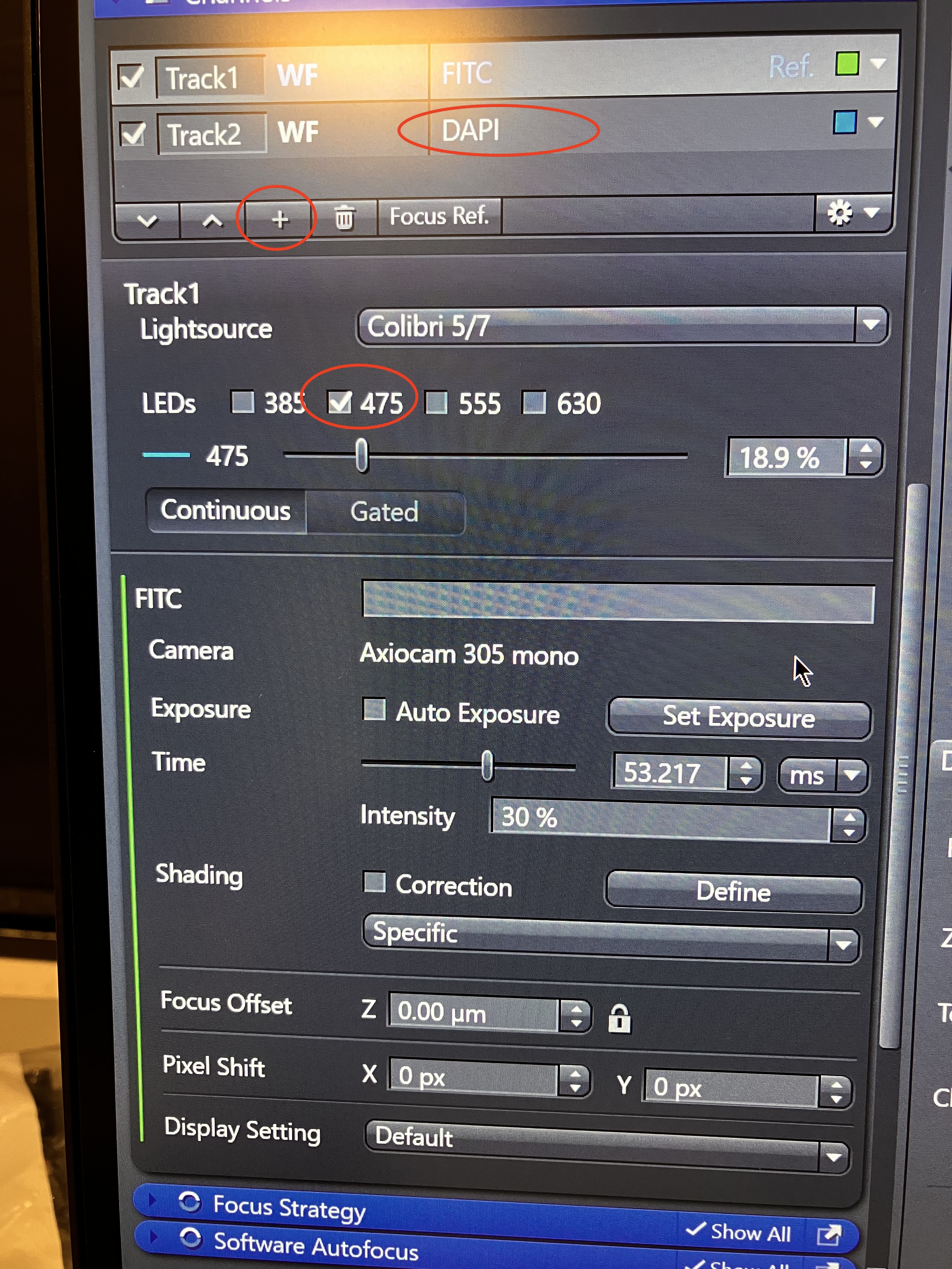
- Scroll down to “Channels” on the left side of your screen. If there are tracks there, you can either delete them or alter them.
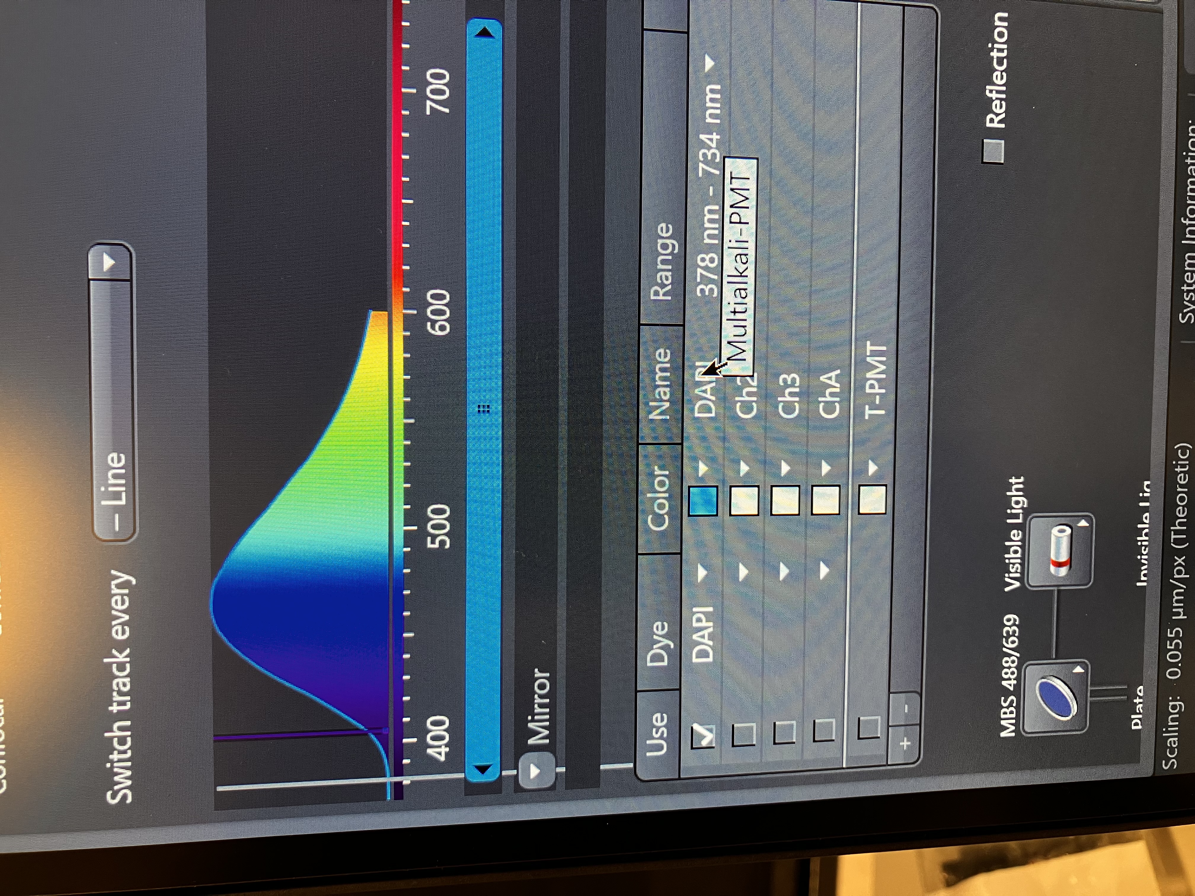
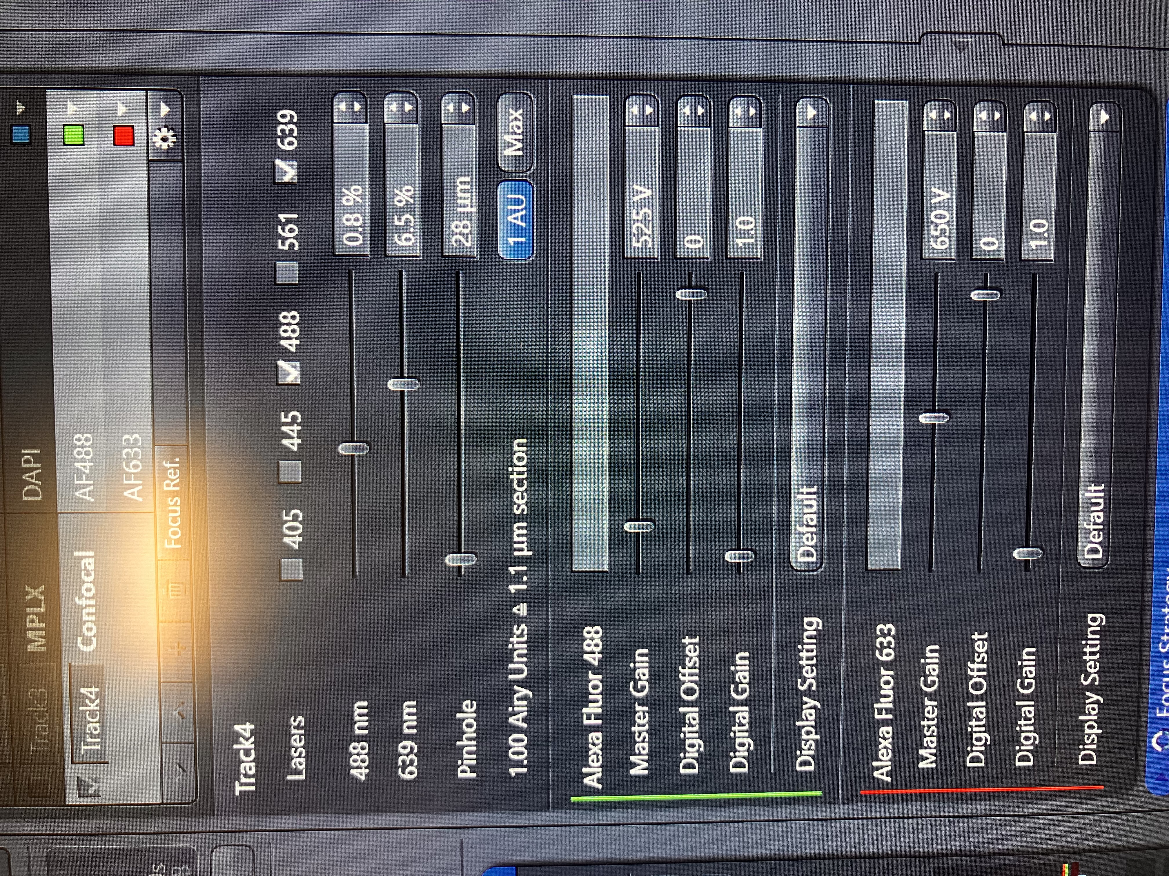
- Add the specific tracks you want, specify the dye for each, and check the corresponding laser for each:
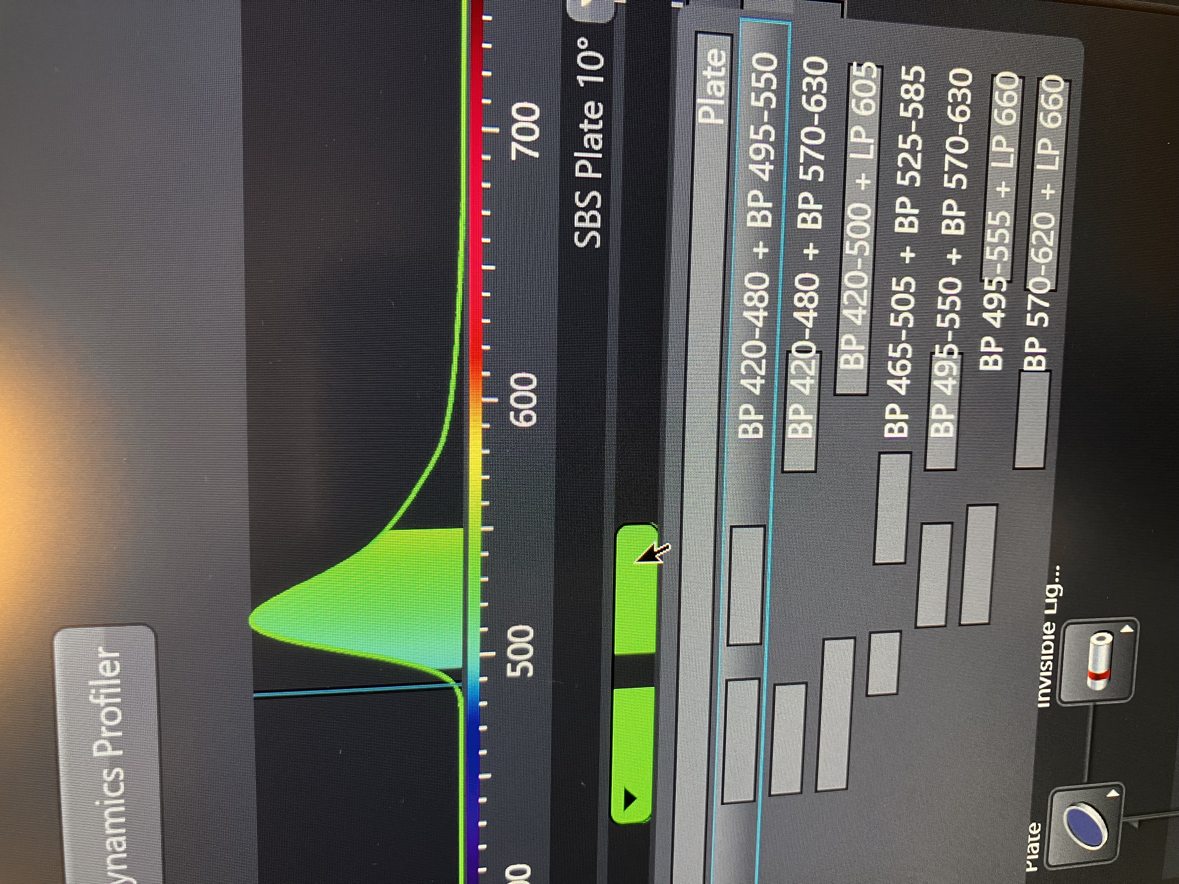
- Adjust the filters for each:
- Important Notes:
Unlike in SR mode, in confocal mode you can adjust the filters in a continuous manner.
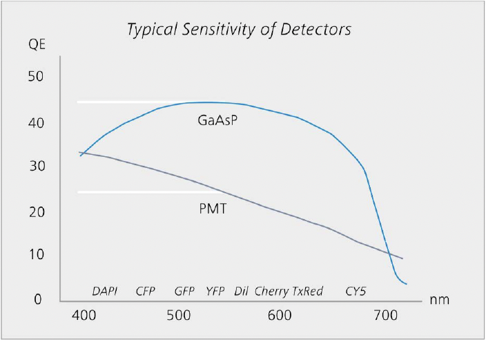
In confocal mode, you can specify which detector is used for each track. Our setup has three detectors: Multialkali-PMTs (assigned to channels 1 and 3), a GaAsP-PMT (assigned to channel 2), and the Airyscan detector (assigned to channel 4). The ladder two are more sensitive, so take fact that into consideration, using this plot:
- As mentioned above, you can perform simultaneous acquisition in confocal mode. Within a track, you can add multiple dyes and adjust the corresponding filters accordingly:
- You can also adjust these dyes’ view settings separately, despite them being in the same track:
3.2.2 Adjust Your Acquisition Scheme
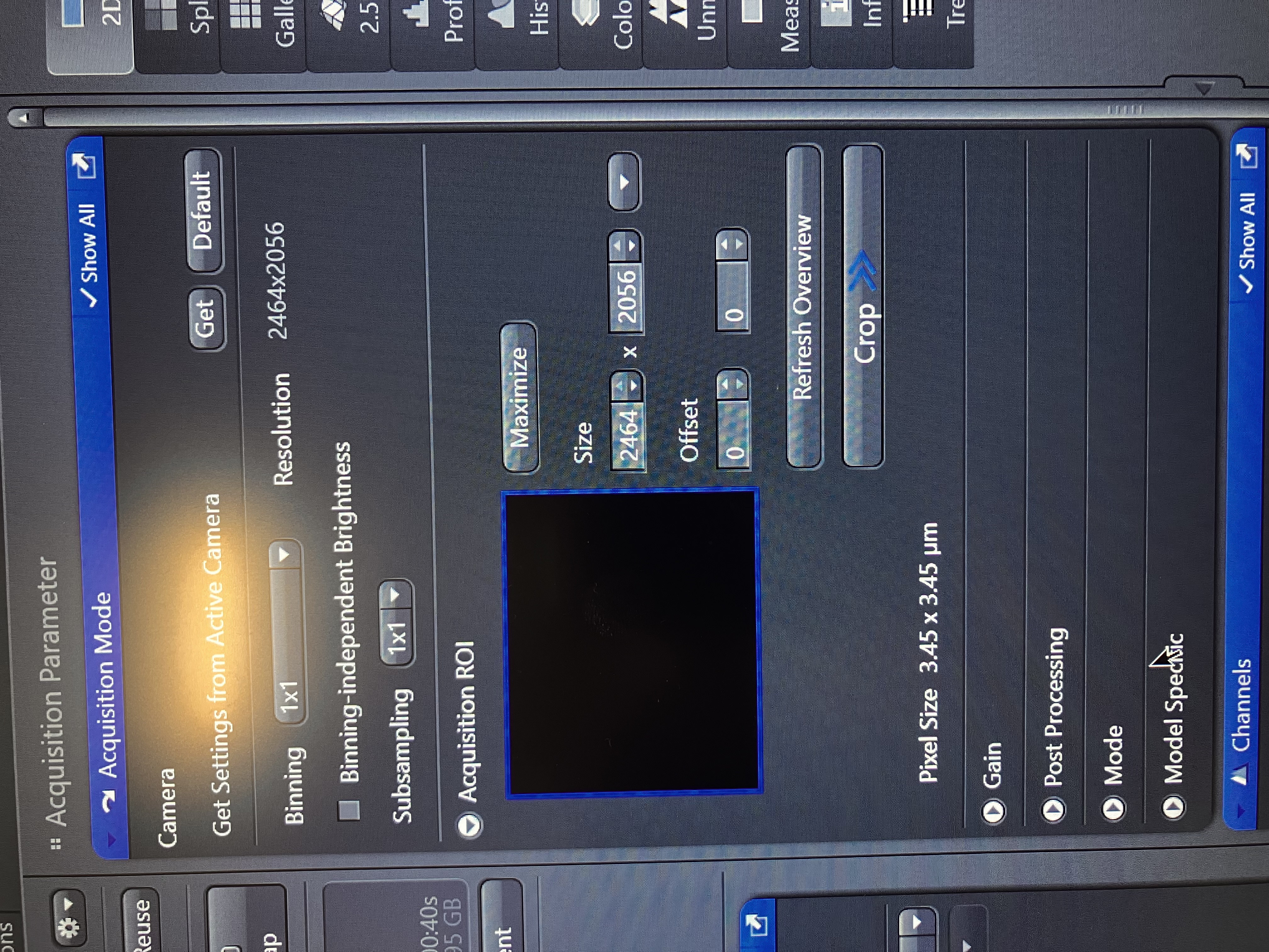
- You may want to customize some settings in the acquisition part:
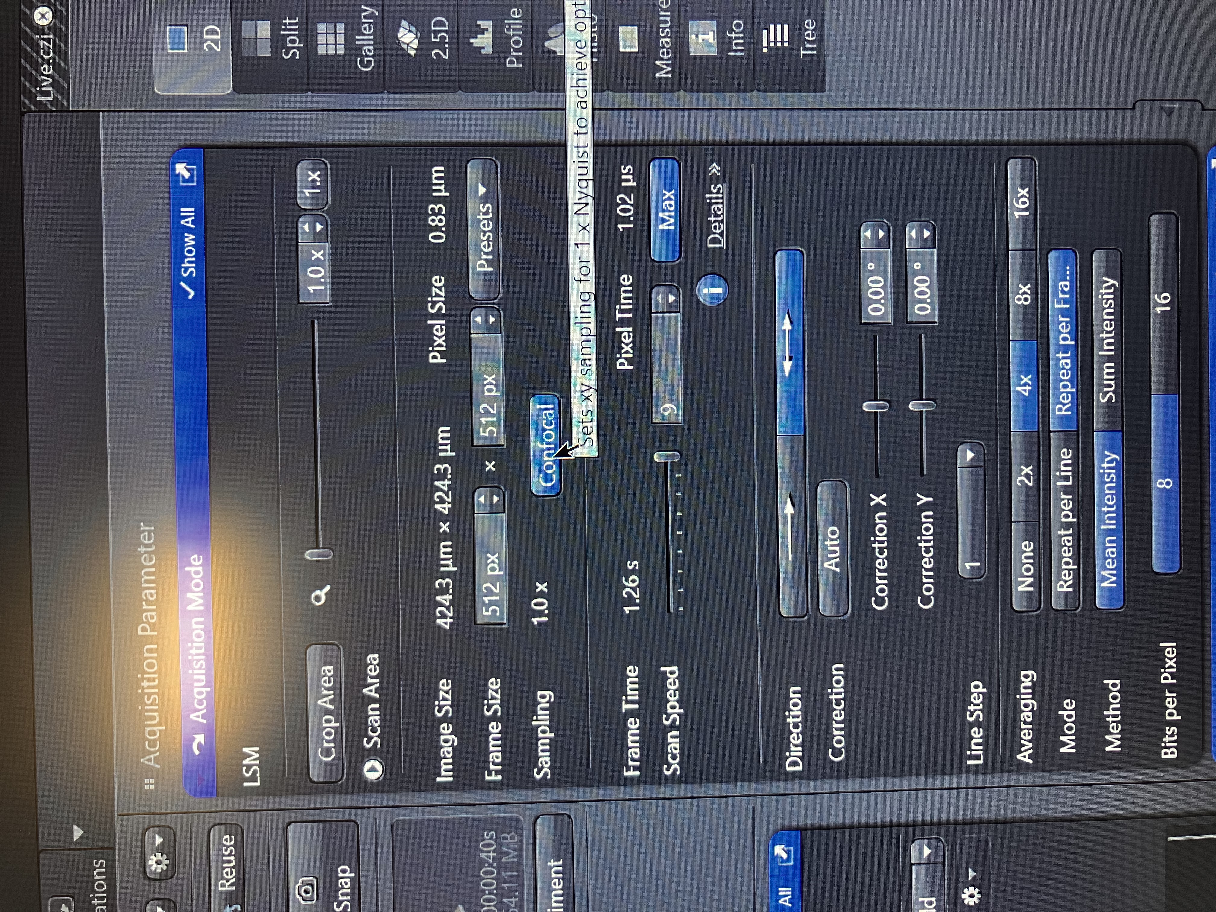
- Crop area refers to the field of view. By default, it is set to 1x. However, you can increase this number to crop the field of view. Frame size refers to the number of pixels that will comprise the image. In “Live” mode, this is set to 512 x 512. “Continuous” mode uses the parameter that you set here. The “Confocal” button ensures that the sampling will achieve Confocal-level resolution.
- Something to pay attention to in the channel part is if you are using “Frame” or “Line” track switching (shown in the previous step).
- Frame means that the entire frame will be scanned and imaged for each track in a sequence. Line means that each line of the frame will be imaged for each track in a sequence.
- Remember that each time the track changes, the laser and/or the filters must switch inside of the machine (unless no changes are necessary). So, if you have tracks with different filters and different lasers, if you use line mode, then many switches must occur at the end of each line of the frame. For a large frame, this can be time consuming.
- Balance your acquisition scheme to achieve quality imaging in a reasonable amount of time (i.e. without much switching). This does not always mean that frame is the best choice because there are usually fewer switches. If you can keep the filters the same for each track, and if you are not dealing with excitation bleed through (see Imaging Considerations), then line is often the better choice.
3.2.3 Ensure You Can See Something & Get in Focus
- Ensure that the stage is at the position that you saved during the setup procedure by tapping “Pos. 2” on the touch pad.
- Select a track and then click “Live.” You should see at least some signal.
The optical system has slightly changed because you changed detectors when you selected confocal. So, the focus is off by a small amount.
- Scan up and down with the fine focus knob or with the computer by scrolling with the mouse while holding the “control” key.
- Stop scanning where the signal is brightest. Note that the focal plane is very thin. Just a fraction of a scroll could reveal the image.
Now, you are in focus in this new optical system with the confocal detector.
3.2.4 Toggle through the Tracks and Optimize View Settings
- For confocal, laser power should be in the loose range of 1 to 5.
- Master gain should be in the loose range of 500 to 900. Digital gain should typically stay set to 1.
Increasing gain will increase the noise of the image. Increasing laser power can cause photo bleaching. Essentially, you want to increase the laser power as much as you know you can without photo bleaching, then adjust the gain accordingly.
- Ensure that the histogram for each track is left skewed and has a range that fills about half or more of the dynamic range. Do not worry about how the image looks yet.
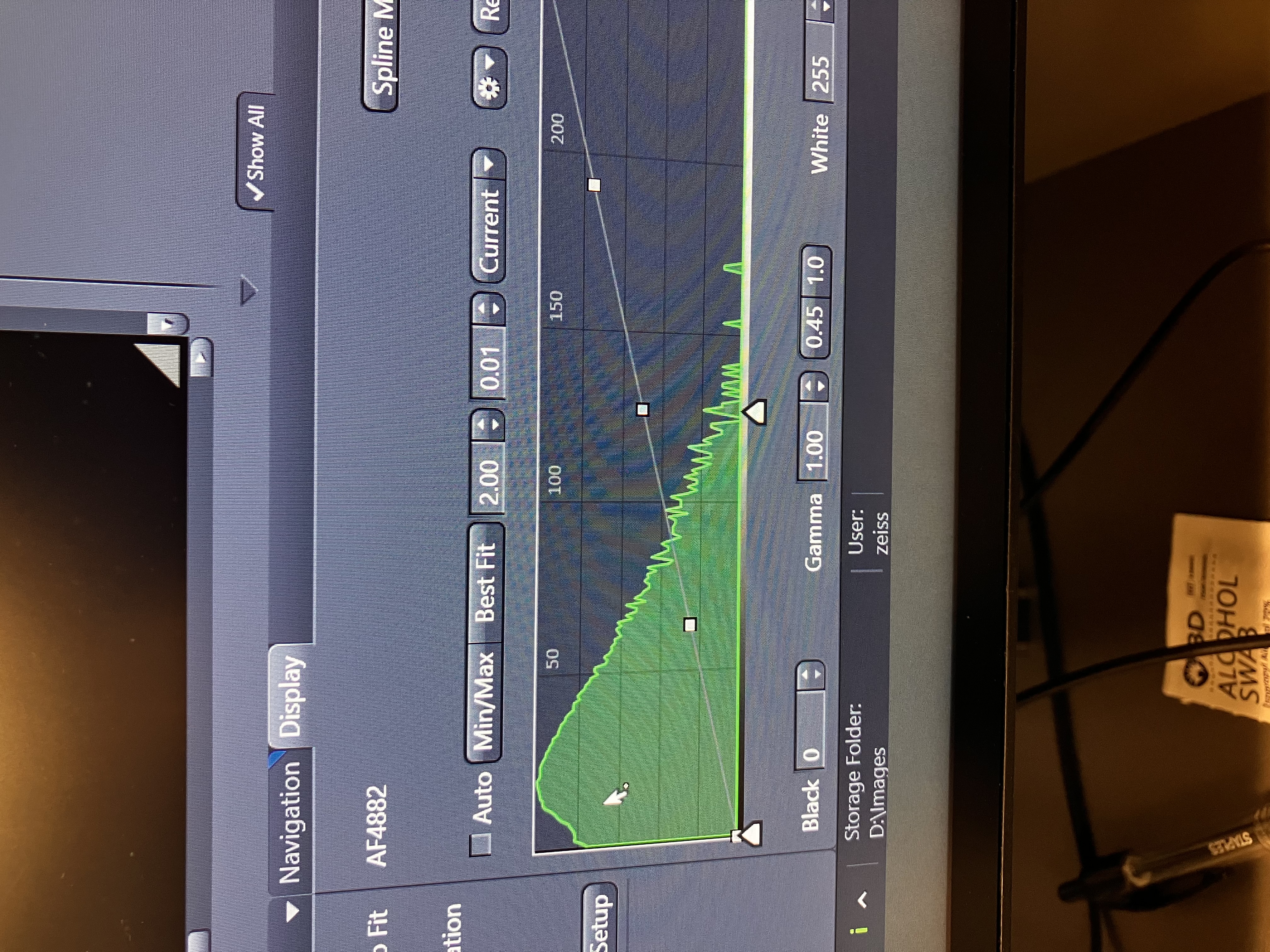
- Check the range indicator for any saturated pixels. There should be no saturated pixels at all. Saturated pixels display as red. Having saturated pixels can negatively affect deconvolution methods in processing steps downstream.
- Stop “Live” mode.
3.3 Widefield Mode
The following outline of steps should get any user a single image acquisition using the widefield modality of this microscope.
Note that if your goal is to accomplish widefield imaging only, you may be using the wrong microscope. Many people use this scope for SR and confocal imaging. It may be more time-efficient, resource-efficient, and cost-efficient for you to use a different microscope that is made for widefield only.
3.3.1 Set Up Tracks and Acquisition Scheme
You can use Smart Setup, load a past setup, or you can do this step manually.
3.3.1.1 Using Smart Setup
- Make sure “WF” is selected.
- Add the fluors you want to image by clicking “+ Dyes & Contrast Methods” and then selecting from the available options. Note that you search for fluors that are not showing up by default.
- Choose the proposal that best suits your needs.
- Click “OK” to finish.
3.3.1.2 Loading a Past Setup
- At the top of the screen on the left side, under “Locate” and “Acquisition,” you can find the name of the current setup. Click on it and toggle to the setup that you would like to load.
3.3.1.3 Manual Setup
- Scroll down to “Channels” on the left side of your screen. If there are tracks there, you can either delete them or alter them.
- Add the specific tracks you want (left), specify the dye for each (middle), and check the corresponding LED for each (right):
3.3.1.4 Adjusting Your Acquisition Scheme
- You may want to customize some settings in the acquisition tab:
- Size refers to the field of view. By default, it is larger than the field of view in confocal mode. It is determined by the number of pixels that will comprise the image. Lowering the number of pixels will crop the image.
3.3.2 Ensure You Can See Something & Get in Focus
- Ensure that the stage is at the position that you saved during the setup procedure by tapping “Pos. 2” on the touch pad.
- Select a track and then click “Live.” You should see at least some signal.
- Scan up and down with the fine focus knob or with the computer by scrolling with the mouse while holding the “control” key.
- Stop scanning where the signal is brightest. The optical system did not change since you completed the setup procedure, so no refocusing should be necessary. Still, it is good to check.
3.3.3 Toggle through the Tracks and Optimize View Settings the laser power and gain settings for each track.
- For widefield, power should be in the range of 20 to 40 percent (find this right below the LED check box). This is not the intensity, which you should can leave alone.
- You should also change the exposure time, as needed.
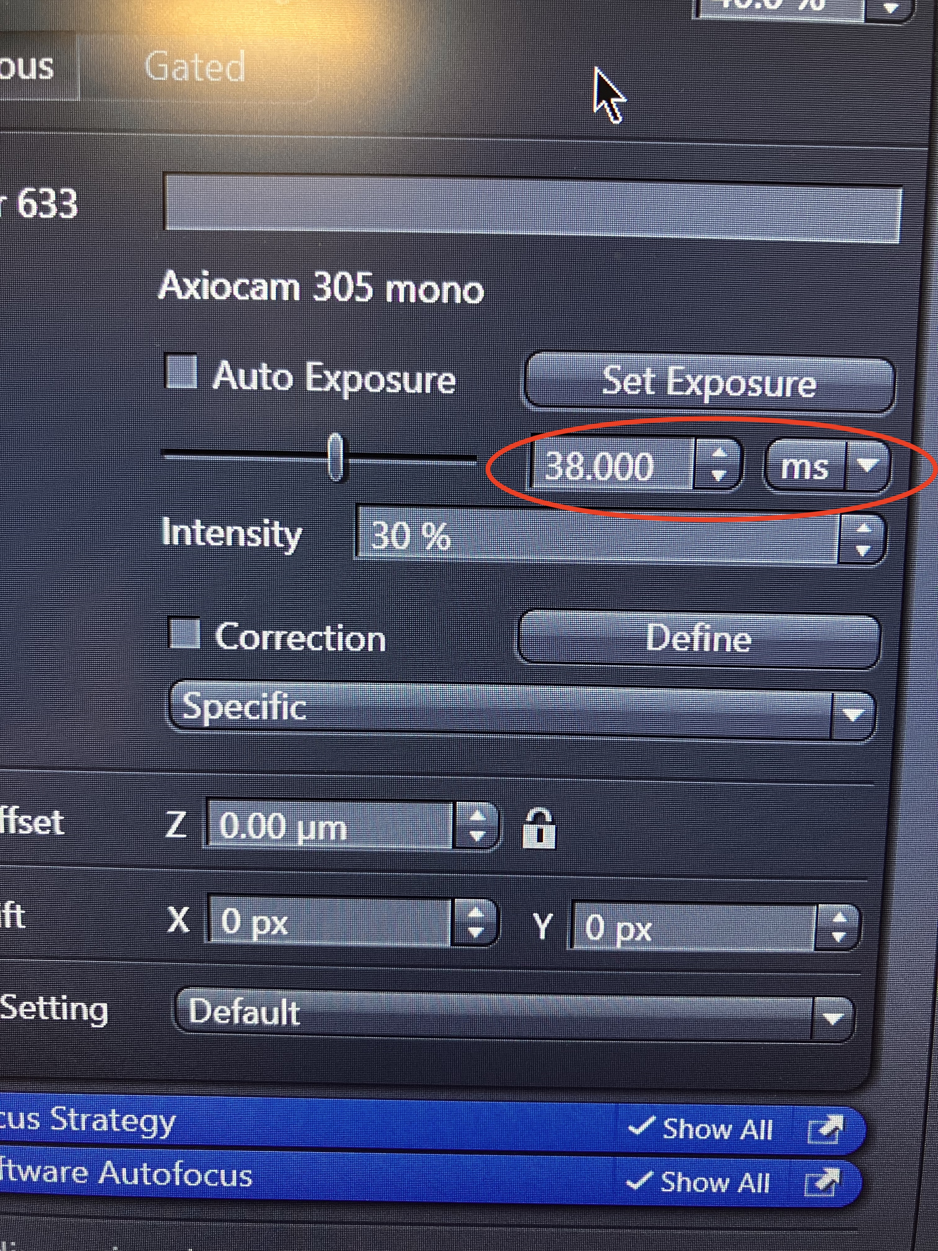
- Gain can be changed here, if needed:
Increasing gain will increase the noise of the image. Increasing LED power and/or exposure can cause photo bleaching. Essentially, you want to increase the power/exposure as much as you know you can without photo bleaching, then adjust the gain accordingly.
- Ensure that the histogram for each track is left skewed and has a range that fills about half or more of the dynamic range.
- Check the range indicator for any saturated pixels. There should be no saturated pixels at all. Saturated pixels display as red. Having saturated pixels can negatively affect deconvolution methods in processing steps downstream.
- Stop “Live.”