Chapter 6 Two-Way ANOVA
6.1 Another Agriculture Example
Since much of the original theory of ANOVA, and a lot of hypothesis testing in general, came from such locations as the Rothamsted Agricultural Station in England (Ronald Fisher worked here) and Iowa State University (one of the first universities in the US to have a separate statistics department), I’ll use another agricultural based example.
In the last chapter, we looked at the completely randomized design or \(CRD\), where there was only a single factor, which in an experiment is controlled via randomization. Often, though, there will exist another factor that is important in terms of explaining the variation in the response variable. That factor may be known but is not something that can be experimentally controlled or manipulated. For example, in a medical study we might be able to control who receives the treatment versus the placebo, but if a variable such as sex is also important, we might choose to use it in the model even though we cannot randomly assign somebody a value for sex the way we could for the treatment.
Turning back to an agricultural example, suppose farmers would like to grow more wheat. Suppose there are \(k=5\) varieties of wheat that could be planted, and we are willing and able to conduct an experiment where different fields are randomly assigned different varieties of wheat to be planted there. Suppose there are \(b=6\) locations (they might be experimental farms) which are inherently different from each other (different soil, different micro-climates, etc.) which we cannot change. What we could do is divide each of the \(b=6\) locations into 5 smaller plots of land, and randomly assign one of the \(k=5\) varieties of wheat to each of these plots. The locations are referred to as blocks and this design is called a randomized block design.
For now, we are assuming that there will only be \(n=1\) replicate per combination of variety and location. This limitation will force us to assume that there is no statistically significant interaction between variety and location. For example, it might be the case that a certain variety of wheat is well suited to the type of soil found at 2 of the locations, but is poorly suited to the soil at the other 4 locations. In the next chapter, we will allow the replicates \(n>1\) and will study this interaction in more detail.
6.2 The Randomized Block Design model
The randomized block design (RBD) model is given:
\[Y_{ij} = \mu + \alpha_i + \beta_j + \epsilon_{ij}\]
\(i=1,2,\cdots,k\) for the number of levels/treatments, where \(j=1,2,\cdots,b\) for the number of blocks being used. The overall sample size \(N=kb\) and the sample size per treatment/block combination is \(n_{ij}=1\).
\(Y_{ij}\) refers to the observation receiving treatment level \(i\) and is in block \(j\). The parameter \(\mu\) in the model is the overall mean, so \(\bar{Y}_{..}\) would be an estimate of it. The parameters \(\alpha_i\) are the treatments effects due to level \(i\) of the factor, while the \(\beta_j\) parameters are block effects due to being in block \(j\). \(\epsilon_{ij}\) is an error/residual, where \(\epsilon_{ij} \sim N(0,\sigma^2)\).
A test of the null hypothesis \(H_O: \alpha_1 = \alpha_2 = \cdots = \alpha_k\) is of primary interest (can I grow more wheat with variety \(i\)?), and the test of the null hypothesis \(H_O: \beta_1 = \beta_2 = \cdots = \beta_b\) (which block grows more wheat?) is of secondary interest. Typically when a blocking variable is utilized, it is because we expect it to be significant, similar to using a covariate \(X\) in an ANCOVA model that is highly correlated with the response variable \(Y\).
6.3 Sums of Squares
There are now 4 lines of the ANOVA table and 4 different sums of squares quantities to compute. The formulas are obviously dreadful to use for hand computations and such calculations will be relegated to the computer.
\[\text{Sum of Squares Total:} \: \: SSY = \sum_{i=1}^k \sum_{j=1}^b (Y_{ij}-\bar{Y}_{..})^2\]
\[\text{Sum of Squares Treatment:} \: \: SSA = b \sum_{i=1}^k (\bar{Y}_{i.}-\bar{Y}_{..})^2\]
\[\text{Sum of Squares Block:} \: \: SSB = k \sum_{j=1}^b (\bar{Y}_{.j}-\bar{Y}_{..})^2\] \[\text{Sum of Squares Error:} \: \: SSE = \sum_{i=1}^k \sum_{j=1}^b (\bar{Y}_{ij}-\bar{Y}_{i.}-\bar{Y}_{.j}+ \bar{Y}_{..})^2\] Once these sums of squares are computed, arrange in a table.
| Source | \(df\) | \(SS\) | \(MS\) | \(F\) | \(p\)-value |
|---|---|---|---|---|---|
| Treatment | \(k-1\) | \(SSA\) | \(MSA\) | \(MSA/MSE\) | \(F(A) \sim F(k-1,(k-1)(b-1))\) df |
| Block | \(b-1\) | \(SSB\) | \(MSB\) | \(MSB/MSE\) | \(F(B) \sim F(b-1,(k-1)(b-1))\) df |
| Error | \((k-1)(b-1)\) | \(SSE\) | \(MSE\) | ||
| Total | \(kb-1\) | \(SSY\) |
6.4 Using R
In my wheat example, there are \(k=5\) varieties of wheat, our treatment, that is the factor of main interest. There are \(b=6\) blocks, which are different locations of experimental farms. We have a total of \(N=kb=30\) plots available for use, and the response variable \(Y\) is a measure of yield (bushels/acre) of the wheat crop. Since I indicated location with numbers rather than letters, I’ll turn it into a factor called block. Even though it is still represented by numbers, they will now be treated categorically (non-numerically).
require(tidyverse)
require(mosaic)
URL <- "https://campus.murraystate.edu/academic/faculty/cmecklin/STA565/wheat.txt"
wheat <- read.table(URL,header=TRUE) %>%
   mutate(block=as_factor(location))
str(wheat)
## 'data.frame': 30 obs. of 4 variables:
## $ variety : chr "A" "A" "A" "A" ...
## $ location: int 1 2 3 4 5 6 1 2 3 4 ...
## $ yield : num 35.3 31 32.7 36.8 37.2 33.1 33.7 32.2 31.4 32.7 ...
## $ block : Factor w/ 6 levels "1","2","3","4",..: 1 2 3 4 5 6 1 2 3 4 ...## variety location yield block
## Length:30 Min. :1.0 Min. :30.70 1:5
## Class :character 1st Qu.:2.0 1st Qu.:32.48 2:5
## Mode :character Median :3.5 Median :33.70 3:5
## Mean :3.5 Mean :34.18 4:5
## 3rd Qu.:5.0 3rd Qu.:36.08 5:5
## Max. :6.0 Max. :38.30 6:5## variety min Q1 median Q3 max mean sd n missing
## 1 A 31.0 32.800 34.20 36.425 37.2 34.35000 2.471235 6 0
## 2 B 31.4 32.325 33.20 33.700 35.0 33.11667 1.279714 6 0
## 3 C 32.2 33.450 35.35 37.250 38.2 35.30000 2.520317 6 0
## 4 D 32.9 35.200 35.60 36.075 38.3 35.61667 1.749762 6 0
## 5 E 30.7 30.975 31.80 33.525 36.1 32.53333 2.117231 6 0## block min Q1 median Q3 max mean sd n missing
## 1 1 32.2 32.4 32.9 33.7 35.3 33.30 1.258968 5 0
## 2 2 30.9 31.0 32.2 33.4 36.1 32.72 2.146392 5 0
## 3 3 31.2 31.4 32.7 33.6 35.2 32.82 1.652876 5 0
## 4 4 30.7 32.7 36.8 37.1 38.3 35.12 3.249923 5 0
## 5 5 33.9 35.0 35.2 37.2 37.3 35.72 1.482228 5 0
## 6 6 33.1 33.7 36.0 36.1 38.2 35.42 2.053534 5 0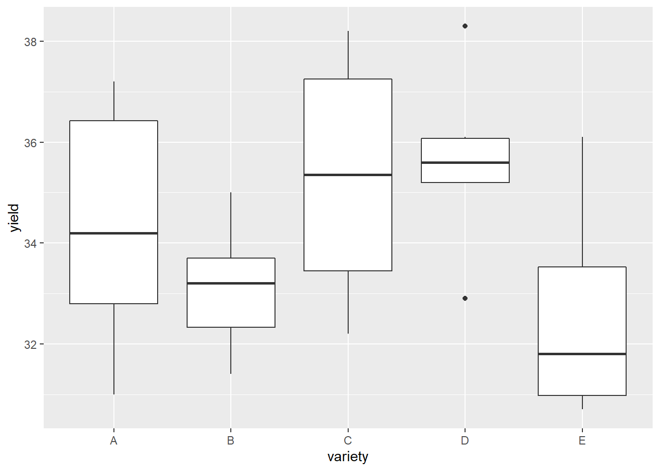
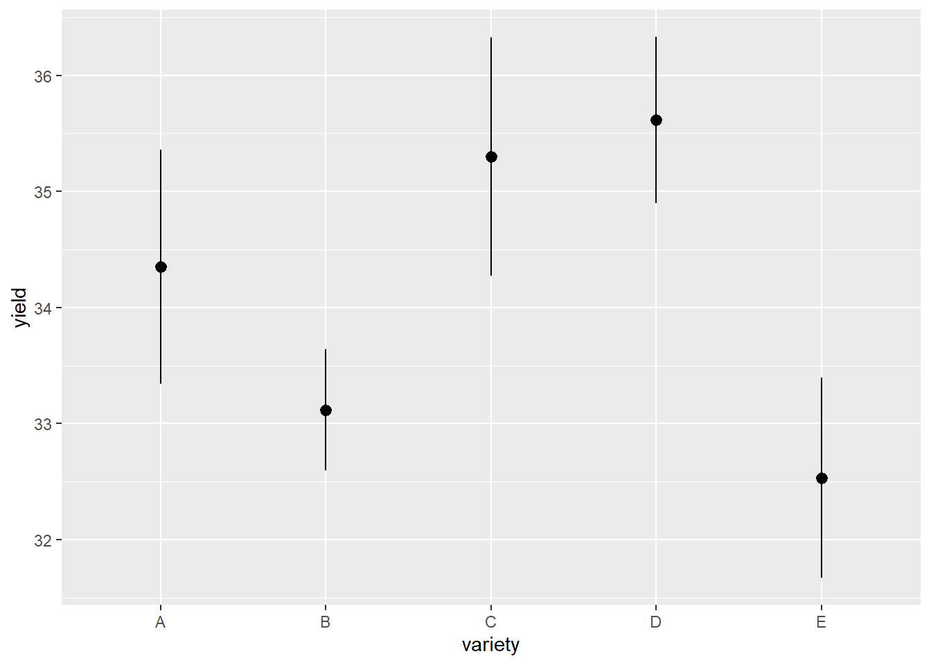
Visually, it looks like varieties C and D are best for maximizing yield, with B and E the worst.
I’ll fit both the one-way ANOVA model that ignores block and the randomized block design model that includes block.
## Analysis of Variance Table
##
## Response: yield
##           Df  Sum Sq Mean Sq F value  Pr(>F)
## variety    4  43.137 10.7842  2.4916 0.06884 .
## Residuals 25 108.205  4.3282
## ---
## Signif. codes: 0 '***' 0.001 '**' 0.01 '*' 0.05 '.' 0.1 ' ' 1## Analysis of Variance Table
##
## Response: yield
## Df Sum Sq Mean Sq F value Pr(>F)
## variety 4 43.137 10.7842 3.5672 0.02368 *
## block 5 47.742 9.5483 3.1584 0.02915 *
## Residuals 20 60.463 3.0232
## ---
## Signif. codes: 0 '***' 0.001 '**' 0.01 '*' 0.05 '.' 0.1 ' ' 1## Tukey multiple comparisons of means
## 95% family-wise confidence level
##
## Fit: aov(formula = yield ~ variety + block, data = wheat)
##
## $variety
## diff lwr upr p adj
## B-A -1.2333333 -4.2372396 1.7705729 0.7353557
## C-A 0.9500000 -2.0539062 3.9539062 0.8752616
## D-A 1.2666667 -1.7372396 4.2705729 0.7164197
## E-A -1.8166667 -4.8205729 1.1872396 0.3956416
## C-B 2.1833333 -0.8205729 5.1872396 0.2292247
## D-B 2.5000000 -0.5039062 5.5039062 0.1326945
## E-B -0.5833333 -3.5872396 2.4205729 0.9763755
## D-C 0.3166667 -2.6872396 3.3205729 0.9976651
## E-C -2.7666667 -5.7705729 0.2372396 0.0802528
## E-D -3.0833333 -6.0872396 -0.0794271 0.0424834
##
## $block
## diff lwr upr p adj
## 2-1 -0.58 -4.0365347 2.876535 0.9943597
## 3-1 -0.48 -3.9365347 2.976535 0.9976778
## 4-1 1.82 -1.6365347 5.276535 0.5743959
## 5-1 2.42 -1.0365347 5.876535 0.2804444
## 6-1 2.12 -1.3365347 5.576535 0.4150325
## 3-2 0.10 -3.3565347 3.556535 0.9999990
## 4-2 2.40 -1.0565347 5.856535 0.2884094
## 5-2 3.00 -0.4565347 6.456535 0.1130653
## 6-2 2.70 -0.7565347 6.156535 0.1848331
## 4-3 2.30 -1.1565347 5.756535 0.3304773
## 5-3 2.90 -0.5565347 6.356535 0.1338006
## 6-3 2.60 -0.8565347 6.056535 0.2156037
## 5-4 0.60 -2.8565347 4.056535 0.9934041
## 6-4 0.30 -3.1565347 3.756535 0.9997603
## 6-5 -0.30 -3.7565347 3.156535 0.9997603Notice in this problem, variety would not be considered significant from the one-way ANOVA model at \(\alpha=0.05\), but it is in the blocking model. Even though it cost us several degrees of freedom to control for the farm’s location (i.e. the block), it was beneficial. We can then follow up with a Tukey’s HSD or other multiple comparison procedure. An even better idea would be to have multiple replicates per cell (i.e. combination of the factors), which is the topic of the next chapter.