Chapter 5 One-Way ANOVA
5.1 Introduction/Assumptions
A common problem in statistics is to test the null hypothesis that the means of two or more independent samples are equal.
When there are exactly two means, we can use parametric methods such as the independent samples \(t\)-test or a nonparameteric alternative such as the Wilcoxon Rank Sum test.
However, when we have more than two samples, these tests do not hold. In this chapter, we will study problems that can be solved with a method based on partioning the variation of a response variable into its components, known as the analysis of variance, or ANOVA.
One of the many problems that can be solved with ANOVA methods is testing for the equality of two or more independent means. This is called one-way ANOVA, as there is a single explanatory variable or factor (sometimes the independent variable).
In order to utilize ANOVA methods, the following assumptions are made:
The data come from two or more independent random samples.
The response (or dependent) variable is normally distributed.
The variance \(\sigma^2\) of each group is equal.
Small deviations from normality are not problematic (although we could use Kruskal-Wallis). Generally, we prefer to have 5 or more observations per level.
Having equal sample sizes (a balanced design) in each group is useful, both for meeting these assumptions and to make calculations easier.
5.2 Cooking Pot Example
There was anecdotal evidence that some people from an African nation were suffering from iron deficiency and a hypothesis was formed that the reason for the deficiency was the type of material that a cooking pot was made out of.
An experiment was designed in which 4 batches of a porridge that is a staple of the diet in this nation were cooked for 3 different types of pot: aluminum, clay, and iron.
The dependent or response variable in this problem is the iron content (measured in mg per 100 g of food) of the porridge.
The independent variable, or factor, in this problem is the type of material the pot is made from. There are \(k=3\) levels (possible values) of this categorical variable.
The type of material is the only factor that is being controlled by the researchers, so we have a one-way ANOVA design. This design is balanced because we have \(n_i=4\) replications per level.
Data Table
| \(i\) | Material | \(n_i\) | Iron Content, \(y_{ij}\) | \(y_{i.}\) | \(\bar{y}_{i.}\) | \(s_i\) |
|---|---|---|---|---|---|---|
| 1 | Aluminum | 4 | \(1.77 \qquad 2.86 \qquad 1.96 \qquad 2.14\) | 8.73 | 2.1825 | 0.4763 |
| 2 | Clay | 4 | \(2.27 \qquad 1.28 \qquad 2.48 \qquad 2.68\) | 8.71 | 2.1775 | 0.6213 |
| 3 | Iron | 4 | \(5.27 \qquad 5.17 \qquad 4.06 \qquad 4.22\) | 18.72 | 4.6800 | 0.6283 |
\[n=\sum_{i=1}^3 n_i=4+4+4=12\]
The sum of all \(n=12\) observations is \(y_{..}=36.16\)
The overall mean is \(\bar{y}_{..}=36.16/12=3.0133\).
5.3 One-Way ANOVA Model
We wish to test the hypotheses \[H_o: \mu_1=\mu_2=\mu_3\] versus \[H_a: \mu_i \neq \mu_j \text{ for at least one } i \neq j\]
One possible mathematical description of the one-way ANOVA model is: \[y_{ij}=\mu + \alpha_i + \epsilon_{ij}\]
In the above model, \(i=1,2,\cdots,k\). In the cooking example \(k=3\) for the three types of cooking pot. An independent samples \(t\)-test is actually just a special case of one-way ANOVA where \(k=2\).
\(j=1,2,\cdots,n_i\). In a balanced design, all \(n_i\) are equal. In the cooking problem \(n_1=n_2=n_3=4\).
\(y_{ij}\) is the jth measurement of the response variable from the ith level of the factor. For example, \(y_{23}=2.48\) (the 3rd measurement from Clay).
\(\alpha_i\) is the effect of the ith treatment level. If the null hypothesis is true, all \(\alpha_i=0\).
\(\epsilon_{ij}\) is the variation for that observation not accounted for by the treatment.
5.4 Sums of Squares
The concept behind ANOVA is to take the total variation in the response variable and to break it up into additive components.
In one-way ANOVA, the total variation is broken up into two components: between-groups variation (i.e. what the model explains) and within-groups variation (i.e. what the model does not explain, often called the error or residual).
Sums of squares are computed from the data. The sum of squares between, or \(SSB\) is often called \(SSM\) (sum of squares mean). The sum of squares within, or \(SSW\) is often called \(SSE\) (sum of squared errors).
\[\text{Sum of Squares Total = SS Mean + SS Error}\]
\[\text{SST = SSM + SSE}\]
\[\sum_{i=1}^k \sum_{j=1}^{n_i} (y_{ij}-\bar{y}_{..})^2 = \sum_{i=1}^k n_i(\bar{y}_{i.}-\bar{y}_{..})^2 + \sum_{i=1}^k \sum_{j=1}^{n_i} (y_{ij}-\bar{y}_{i.})^2\]
Here, I will compute the , or \(SST\), for the cooking example, using an algebraically equivalent formula. \[SST=\sum_{i=1}^k \sum_{j=1}^{n_i} (y_{ij}-\bar{y}_{..})^2 = \sum_{i=1}^k \sum_{j=1}^{n_i} y_{ij}^2 -\frac{(y_{..})^2}{n}\] \[SST=(1.77^2+2.36^2+\cdots+4.22^2)-\frac{(36.16)^2}{12}\] \[SST=128.6516-108.9621\] \[SST=19.6895\]
Notice that \(SST\) is merely the numerator of the formula for sample variance.
Now I will compute the sum of squares mean, or \(SSM\) for the cooking example. This term is often called sum of squares between, treatment or model.
\[SSM=\sum_{i=1}^k n_i(\bar{y}_{i.}-\bar{y}_{..})^2\]
\[SSM=4(2.1825-36.16/12)^2+4(2.1775-36.16/12)^2\]
\[+4(4.68-36.16/12)^2\]
\[SSM=16.66672\]
When this term is large relative to \(SST\), that indicates that there is a significant effect due to the factor.
The sum of squares error \(SSE\) (often called sum of squares within or residual) is the most tedious sum of squares term to compute, so we typically find it by subtraction after finding \(SST\) and \(SSM\).
\[SST=SSM+SSE\]
\[19.6895=16.66672+SSE\]
\[SSE=2.5328\]
Another formula for computing \(SSE\) is useful when we only know the means and standard distributions of the treatments.
\[SSE=\sum_{i=1}^k (n_i-1)s_i^2\]
\[SSE=3(.2520)^2+3(.6213)^2+3(.6283)^2\]
\[SSE=3.02278\]
5.5 The ANOVA Table
These sums of squares terms are then typically arranged in a tabular format called the ANOVA table.
Each row of the ANOVA table represents a source of variation; for one-way ANOVA we have model, error, and total variation.
The columns of the ANOVA table contain the sum of squares (\(SS\)) for each source of variation, along wiht the degrees of freedom (\(df\)), the mean square (which is just \(MS=SS/df\)), an \(F\) ratio that serves as the test statistic, and a \(p\)-value for the test.
General Format of the Balanced One-Way ANOVA Table
| Source | \(df\) | \(SS\) | \(MS\) | \(F\) | \(p\)-value |
|---|---|---|---|---|---|
| Mean | \(k-1\) | \(SSM\) | \(MSM\) | \(MSM/MSE\) | \(P(F>F^*)\) |
| Error | \(n-k\) | \(SSE\) | \(MSE\) | ||
| Total | \(n-1\) | \(SST\) |
In the above table, \(k\) is the number of levels in the factor, \(n\) is the overall sample size, \(SSM,SSE,SST\) are sums of squares and \(MSM,MSE\) are mean squares.
The test statistic is \(F=\frac{MSM}{MSE}\).
If the null hypothesis is true, then both \(MSM\) and \(MSE\) are independent estimates of the variability in the response, or \(\sigma^2\) and \(F=1\). When there is a significant effect due to the factor, then \(MSM>MSE\) and hence \(F>1\).
To determine statistical significance, we can look up the critical value \(F^*\) from the F distribution table using a table or the R function qf, using confidence level \(1-\alpha\), and \(k-1\) & \(n-k\) degrees of freedom. Technology will compute the \(p\)-value, which is compared to \(\alpha\) in the usual way.
In the cooking problem, \(k=3\) and \(n=12\).
| Source | \(df\) | \(SS\) | \(MS\) | \(F\) | \(p\)-value |
|---|---|---|---|---|---|
| Mean | 2 | 16.66672 | 8.33336 | 24.81168 | \(0.0002\) |
| Error | 9 | 3.02278 | 0.3358644 | ||
| Total | 11 | 19.68950 |
The test statistic, or \(F\)-ratio, is \(F=\frac{8.33336}{0.3358644}=24.81168\)
Since the \(F\)-ratio is much larger than 1, we probably have a significant result.
The critical value \(F^*\) can be found.
## [1] 4.256495Since \(F>F^*\), we reject the null hypothesis at \(\alpha=0.05\) and conclude that there is a significant effect on mean iron content between the different cooking pots.
With a TI calculator, \(p\)-value=Fcdf(24.81168,9999999,2,9) \(=0.0002\).
With R, the \(p\)-value is:
## [1] 0.00021765725.6 One-WAY ANOVA with R
This analysis can be easily performed with R. I’ll use direct data entry for this problem.
require(tidyverse)
require(mosaic)
material <- c(rep("Aluminum",4),rep("Clay",4),rep("Iron",4))
iron.content <- c(1.77,2.86,1.96,2.14,
                  2.27,1.28,2.48,2.68,
                  5.27,5.17,4.06,4.22)
cooking.pot <- data.frame(material,iron.content)

favstats(iron.content~material,data=cooking.pot)
## material min Q1 median Q3 max mean sd n missing
## 1 Aluminum 1.77 1.9125 2.050 2.320 2.86 2.1825 0.4762615 4 0
## 2 Clay 1.28 2.0225 2.375 2.530 2.68 2.1775 0.6213091 4 0
## 3 Iron 4.06 4.1800 4.695 5.195 5.27 4.6800 0.6282781 4 0Two useful graphs for ANOVA problems are the boxplot and the error bar plot.
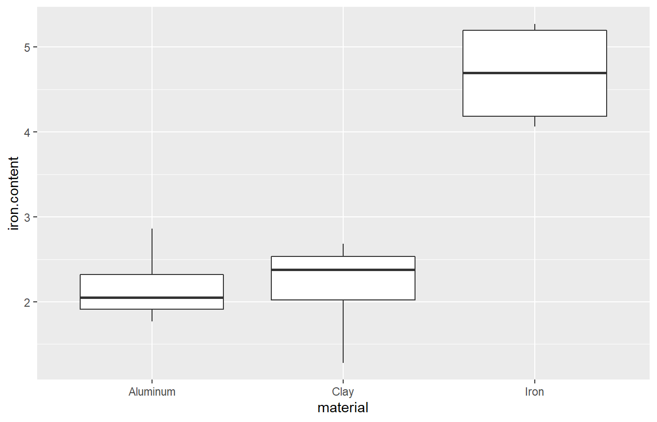
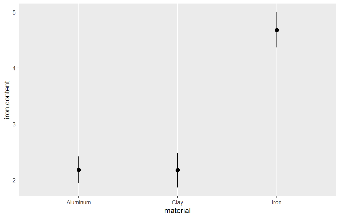
Visually, there seems to be a significant difference between the types of cooking pot, particularly between the iron pots and the other pots. There is very little difference between alumimum and clay.
##             Df Sum Sq Mean Sq F value   Pr(>F)
## material     2 16.667   8.333   24.81 0.000218 ***
## Residuals    9  3.023   0.336
## ---
## Signif. codes:  0 '***' 0.001 '**' 0.01 '*' 0.05 '.' 0.1 ' ' 1
In the cooking problem, we have found a significant effect on the iron content of the porridge due to the type of cooking pot that is used.
Visually, the boxplot and the error bar plot seem to indicate that the iron content is much higher when iron pots are used as oppposed to aluminum or clay, while the difference between aluminum and clay is minor.
To answer this question statistically, we will use what are known as either multiple comparisons or post hoc tests. (chapter 8)