Chapter 12 Classical Nonparametric Statistics

In the previous chapters, we have studied statistical inference, both in the form of confidence intervals and hypothesis tests. The majority of the methods that we have covered assume that the sample data follow some sort of probability distribution (usually the normal) and are often called parametric methods.

In this chapter, we will look at nonparametric hypothesis tests for a variety of situations. These tests make fewer assumptions about that data, are often based on ranking the data, and the hypotheses often involve medians, rather than means.

Some of the advantages of nonparametric tests are:

They can be used in situations where the assumptions of parametric tests (such as normality) are known to be violated.
They can be used in situations where the sample sizes are small. In this situation, it is difficult to assess the normality of the data and the Central Limit Theorem can not be applied.
The theory behind the rank-based nonparametric procedures covered in this chapter is relatively simple.

Of course, there are disadvantages as well:

Applying a nonparametric test will often require the use of specialized tables or computer software which may not be available.
These procedures are not available on the TI-83/84 calculators, which are designed for statistical procedures studied in a STAT 101 or AP Stats class.
Most importantly, nonparametric tests will have LESS POWER when used in situations where the parametric tests are appropriate.

12.1 The Signed-Rank Test

A very basic procedure known as the sign test (details not covered) is rather ‘wasteful’ in the way it uses data. It only looks at the sign or the direction of a difference and ignores its magnitude. For example, a dieter who lost 1 pound and a dieter who lost 25 pounds are both reduced to a single \(\textbf{+}\). They are treated as if their weight loss was the same.
Frank Wilcoxon developed a number of nonparametric tests in the 1940s. In his procedures, we will consider not just the direction, but the rank of a difference.
Wilcoxon’s procedure based on signed ranks is more powerful than the sign test for one-sample or paired-samples problems.

We will consider an example involving people who are trying to lose weight by dieting.

Step One: Write Hypothesis \[H_O: M_D=0\] \[H_A: M_D>0\]

The null hypothesis states that the median difference in weight loss is zero (i.e. the diet was ineffective). The alternative hypothesis states that the median difference in weight loss is greather than zero (i.e. the diet was effective).

Step Two: Choose Level of Significance Let \(\alpha=0.05\), the standard choice.

Step Three: Choose Test & Check Assumptions

We will use the Signed-Rank test. We have a random sample and the differences in the paired data come from a continuous distribution. This second condition is a slightly stronger assumption than in the sign test. With ordinal level differences (i.e. we have +s and -s and no numerical values), the sign test would be the only appropriate choice.

Notice that we are using the Wilcoxon Signed-Rank Test in a situation where we would have considered use of the paired samples \(t\)-test.

Step Four: Calculate the Test Statistic

In the Signed-Rank test, we take the absolute value of the difference, rank those absolute difference, attach the appropriate sign (+ or -), and sum the positive and negative signed ranks. The smallest absolute difference is assigned a rank of 1, the second smallest a rank of 2, and so forth until the largest absolute difference receives a rank of \(n\).

If you have tied absolute difference, assign the average rank. For example, if both the third and fourth smallest absolute difference were 5, both would be assigned a rank of \(\frac{3+4}{2}=3.5\).

We remove data points where the difference is zero (i.e. neither positive nor negative).

Patient	X	Y	D	Sign	Abs.D	Rank	Signed.Rank
1	220	206	14	+	14	6.0	6.0
2	214	197	17	+	17	7.0	7.0
3	190	190	0	None	NA	NA	NA
4	189	200	-11	-	11	4.5	-4.5
5	182	171	11	+	11	4.5	4.5
6	193	196	-3	-	3	1.0	-1.0
7	209	203	6	+	6	2.0	2.0
8	236	226	10	+	10	3.0	3.0

\(D=X-Y\), or difference is weight before minus weight after

Patient #3 receives no rank since \(|D|=0\).

Patients #4 and #5 both have \(|D|=6\) and end up sharing rank 4 and 5 and are assigned a rank of 4.5. Patient #4 ends up with signed rank -4.5.

\[T^+=\text{Sum of positive signed ranks}=22.5\] \[T^-=\text{|Sum of negative signed ranks|}=|-5.5|=5.5\] \[T=\min(T^+,T^-)=\min(22.5,5.5)=5.5 \]

We have \(T=5.5\) with \(n=7\) and a one-sided alternative. The test statistic given in R is called \(V\) and is found as \[V=\frac{n(n+1)}{2}-T\]

The concept of the Signed-Rank Test is that if the null hypothesis is true and the signed ranks are positive or negative randomly, then we would expect the test statistic to be equal to \(T=\frac{n(n+1)}{4}\). In our case, that value is \(\frac{7(7+1)}{4}=14\). If the test statistic is much larger or smaller than 14, we will reject \(H_O\).

Unlike a parametric test, we do not compare the test statistic to a probability distribution such as the standard normal or \(t\). Instead, for \(4 \leq n \leq 12\), the entire sampling distribution of \(T\) is compiled and \(p\)-values are either found with a specialized table (not given in our book) or with the use of software.

wilcox.test(x=X,y=Y,paired=TRUE,correct=FALSE,alternative="greater")

## 
##  Wilcoxon signed rank test
## 
## data:  X and Y
## V = 22.5, p-value = 0.07503
## alternative hypothesis: true location shift is greater than 0

# what R calls V is what I called T+

Step Five: Find the \(p\)-value

We have \(T=5.5\) with \(n=7\) and a one-sided alternative \(H_A: M_D>0\).
Using R, the test statistic computed is \(V=22.5\) and the \(p\)-value is \(p=0.07503\).
We fail to reject \(H_0\) at \(\alpha=.05\).

Step Six: Conclusion

Since we failed to reject the null hypothesis; a proper conclusion would be:

The dieters did NOT lose a significant amount of weight, or the median difference in weight loss is not significantly greater than zero.

There is no function on the TI-83/84 calculators for the Signed-Rank test, but it is available in R with the wilcox.test function.

12.2 The Normal (Large-Sample) Approximation

If your sample size is \(n \geq 16\), one option would be to make a normal approximation, as described on page 227. You ‘create’ a \(z\)-statistic from \(T\):

\[\mu=\frac{n(n+1)}{4}\] \[\sigma^2=\frac{\mu(2n+1)}{6}\] \[Z=\frac{T-\mu}{\sigma}\]

You then compute the \(p\)-value based on the standard normal distribution.

I would generally NOT use this normal approximation, although I will illustrate it in the next example. This example uses the ArcheryData example to see if there was improvement in archery skills between Day1 and the LastDay of an archery class.

# large sample example (n >=16)
require(Stat2Data)
data(ArcheryData)
wilcox.test(Pair(Day1,LastDay)~1,data=ArcheryData,
            correct=FALSE,alternative="less")

## 
##  Wilcoxon signed rank test
## 
## data:  Pair(Day1, LastDay)
## V = 6, p-value = 0.0002674
## alternative hypothesis: true location shift is less than 0

# use normal approximation
n <- 18
T <- 6 
mu <- n*(n+1)/4
sigma2 <- mu*(2*n+1)/6
Z <- (T-mu)/sqrt(sigma2)
pnorm(q=Z) # very close in this problem

## [1] 0.0002678364

12.3 The WSR Test for One Sample

We will consider an example involving total cholesterol level.

Step One: Write Hypothesis \[H_0: M=180\] \[H_a: M \neq 180\]

The null hypothesis states that the median total cholesterol level is 180, and the alternative is that the median total cholesterol level is different from 180.

Step Two: Choose Level of Significance Let \(\alpha=0.05\), the standard choice.

Step Three: Choose Test & Check Assumptions

We will use the Wilcoxon Signed-Rank test. We have a random sample and the differences in the sample come from a continuous distribution.

Step Four: Compute the Test Statistic We will subtract 180 from each data value and compute the \(T\) statistic.

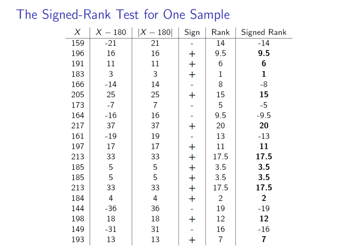
Step Five: Find the \(p\)-value

We have \(T=\min(T^+,T^-)=\min(125.5,84.5)=84.5\) with \(n=20\) and a two-sided alternative \(H_a: M \neq 180\).
Since \(n>12\), I compute the normal approximation. \[\mu=\frac{n(n+1)}{4}=\frac{20(21)}{4}=105\] \[\sigma^2=\frac{\mu(2n+1)}{6}=\frac{105(41)}{6}=717.5\] \[z=\frac{T-\mu}{\sigma}=\frac{84.5-105}{\sqrt{717.5}}=-0.77\]

Step Five: Find the \(p\)-value

The approximate \(p\)-value is \(2P(Z<-0.77)=2(.2206)=.4412\).
We fail to reject \(H_0\) at \(\alpha=0.05\).

Step Six: Conclusion

Since we failed to the null hypothesis; a proper conclusion would be:

The median total cholesterol level is NOT significantly different from 180.

This example, with the wilcox.test function. Again, R uses \(V=T^+\) as the test statistic.

cholesterol <- c(159,196,191,183,166,205,173,164,217,161,197,213,185,
                 185,213,184,144,198,149,193)
wilcox.test(x=cholesterol,mu=180)

## 
##  Wilcoxon signed rank test with continuity correction
## 
## data:  cholesterol
## V = 125.5, p-value = 0.4552
## alternative hypothesis: true location is not equal to 180

12.4 A Nonparametric Test for Two Independent Means

We studied two different versions of the two-sample \(t\)-test for comparing the means of two independent samples. Frank Wilcoxon developed a nonparametric test for this situation, known as the Wilcoxon Rank-Sum Test.
Henry Mann and Donald Whitney, at the same time, developed an essentially identical test called the Mann-Whitney \(U\) Test.
Depending on what book or article you are reading, this test might be called the Rank-Sum Test, Two-Sample Wilcoxon Test, Mann-Whitney \(U\) Test (my preference), or the Wilcoxon-Mann-Whitney Test (giving all three men credit).

Suppose I want to compare the average age of two groups of people. The first group is of size \(n_1=5\) and consists of five people that own an iPhone . The second group is of size \(n_2=6\) and consists of six people that own an Android phone. We want to see if there is a significant difference between the groups.

Notice that these two samples are of different people and are independent of one another, so we will not use a paired-samples method such as the Wilcoxon Signed-Ranked Test.

Step One: Write Hypothesis

\[H_O: P(X_i>Y_j)=0.5 \text{ versus } H_A: P(X_i>Y_j) \neq 0.5\]

The null hypothesis states that the probability that a randomly chosen observation from one population is greater than a randomly chose observation from the other population is 0.5. Alternatively, the null hypothesis states that the two populations are identical versus an alternative that they are shifted from each other.

Informally, think of this as testing the null hypothesis that the two medians (rather than means, as in the \(t\)-test), are equal.

Step Two: Choose Level of Significance

Let \(\alpha=0.05\), the standard choice.

Step Three: Choose Test & Check Assumptions

We will use the Rank-Sum Test. We have 2 independent random samples and the data come from independent continuous distributions.

Step Four: Compute the Test Statistic

In order to compute the test statistic \(T\), we combine the two independent samples into one sample, assign the data values in the combined sample ranks from 1 to \(n=n_1+n_2\), and sum the ranks of the first sample. \(T=\text{Sum(Ranks from Sample 1)}\)

By convention, we define sample 1 to be the smaller of the two samples.

Since \(n_2 \leq 8\), compute \(U=n_1 n_2 + \frac{n_1(n_1+1)}{2}-T\).

The \(p\)-values in the specialized table Table IX on pages 655-656 were determined by considering the \(U\) statistic for all possible arrangements of \(n_1\) ranks from all possible ranks.

\(X\) is the ages of \(n_1=5\) iPhone users and \(Y\) the ages of \(n_2=6\) Android users.

\(X\)	Rank	\(Y\)	Rank
44	8	23	2
52	9	39	7
25	3	33	5.5
33	5.5	53	10
58	11	21	1
		32	4

\[ \begin{aligned} T = & \text{Sum(Ranks from Sample 1)} \\ = & 8+9+3+5.5+11 \\ = & 36.5 \end{aligned} \]

\[ \begin{aligned} U = & n_1 n_2 + \frac{n_1(n_1+1)}{2}-T \\ = & 5(6)+\frac{5(6)}{2}-36.5 \\ = & 30+15-36.5 \\ = & 8.5 \end{aligned} \]

We can easily perform this test in R. R calls the test statistic \(W\) rather than \(U\).

# Wilcoxon Rank-Sum Test aka Mann-Whitney U Test
age <- c(44,52,25,33,58,23,39,33,53,21,32)
phone <- c(rep("iPhone",5),rep("Android",6))
phone.data <- data.frame(age,phone)
wilcox.test(age~phone,data=phone.data)

## 
##  Wilcoxon rank sum test with continuity correction
## 
## data:  age by phone
## W = 8.5, p-value = 0.2722
## alternative hypothesis: true location shift is not equal to 0

# U = 8.5

Step Five: Find the \(p\)-value

We have \(U=8.5\) with \(n_1=5, n_2=6\) and a two-sided alternative \(H_A: M_1 \neq M_2\).
Our \(p\)-value is \(p=0.2722\).
We fail to reject \(H_0\) at \(\alpha=.05\).

Step Six: Conclusion

Since we failed to the null hypothesis; a proper conclusion would be:

The median ages of iPhone users and Android users are not significantly different.

12.5 The Rank-Sum Test, Large Sample

We will reconsider the example for a larger sample. We analyzed this data set in a previous chapter, comparing the exam scores of a class taking their final on Monday versus a class taking their final on Friday.

The data is a file called ExamScores.txt at

http://campus.murraystate.edu/academic/faculty/cmecklin/ExamScores.txt

If we analyze this data with the \(t\)-test for two independent samples, we found no significant difference between the two classes. With Welch’s unequal variances version, we got \(t=-1.7935\) with \(df=24.084\) and \(p=.08547\).

require(tidyverse)
exam.scores <- read.table("http://campus.murraystate.edu/faculty/cmecklin/ExamScores.txt",
                          header=TRUE)
ggplot(exam.scores,aes(x=class,y=exam)) + geom_boxplot()

t.test(exam~class,data=exam.scores)

## 
##  Welch Two Sample t-test
## 
## data:  exam by class
## t = -1.7935, df = 24.084, p-value = 0.08547
## alternative hypothesis: true difference in means between group F and group M is not equal to 0
## 95 percent confidence interval:
##  -21.469922   1.503255
## sample estimates:
## mean in group F mean in group M 
##        68.66667        78.65000

You may recall that the boxplots showed an outlier in the Friday group, that we ignored before. The presence of this outlier, however, with small samples could lead us to choosing the Rank-Sum Test.

Step One: Write Hypothesis \[H_0: Pr(X_i>Y_j)=0.5 \text{ versus } H_a: Pr(X_i>Y_j) \neq 0.5\]

Or, informally:

\[H_0: M_{Monday} = M_{Friday} \text{ versus } H_a: M_{Monday} \neq M_{Friday}\]

Think of this as testing the null hypothesis that the medians of the two groups (rather than means, as in the \(t\)-test), are equal against an alternative that the median of Group 1 (Monday) is different than the median of Group 2 (Friday). I have not specified whether I think the scores are higher on Monday or Friday.

Step Two: Choose Level of Significance

Let \(\alpha=0.05\), the standard choice.

Step Three: Choose Test & Check Assumptions

We will use the Rank-Sum Test. We have 2 independent random samples and the data come from independent continuous distributions.

Step Four: Compute the Test Statistic

Instead of computing the test statistic manually, we will have R compute it for us.

wilcox.test(exam~class,data=exam.scores)

## 
##  Wilcoxon rank sum test with continuity correction
## 
## data:  exam by class
## W = 96.5, p-value = 0.07706
## alternative hypothesis: true location shift is not equal to 0

Step Five: Find the \(p\)-value

From the R output, the test statistic is \(W=96.5\), with \(\text{p-value }=.07706\). We fail to reject the null.
Mann and Whitney used this formula: \[U=[\text{Sum of Ranks of Sample 1}]-\frac{n_1(n_1+1)}{2}\]
In our case, \(U=216.5-\frac{15(16)}{2}=216.5-120=96.5\). R chooses to call this statistic \(W\) rather than \(U\).

Step Six: Conclusion

Since we failed to the null hypothesis; a proper conclusion would be:

The distributions of exam scores are NOT significantly different between the two classes.

This is essentially the same conclusion as we got with the two-sample \(t\)-test, but in using the nonparametric Rank-Sum test instead, the presence of an outlier in the data is not troublesome.

12.6 Comparing the Means of Two or MORE Independent Populations

There are many situations where we would want to compare the means of two or MORE independent populations. For example, we might have 3 groups in a clinical trial: a group receiving a high dose of a drug, a second group receiving a low dose of the drug, and a third group receiving a placebo.
It would be incorrect to just apply \(t\)-tests or Wilcoxon Rank Sum tests to each pair of treatments.
The reason why is that we will INFLATE the chance of committing a Type I Error. With a single test, the Type I Error rate is \(\alpha\).
However, when we run \(t\) independent tests on the same data, the probability of Type I Error rate is \(\alpha=1-(1-\alpha_{NOM})^t\), where \(\alpha_{NOM}\), or nominal alpha is the level of significance that we typically choose, such as 0.05.
With 3 groups, there are three possible pairwise comparisons of means (high-low, high-placebo, low-placebo), and the true Type I Error rate would be \(\alpha=1-(1-0.05)^3=1-.95^3=.143\).
The usual parametric technique for this situation, where \[H_0: \mu_1=\mu_2=\cdots=\mu_k \text { versus } H_a: \text{At least one } \mu_i \neq \mu_j\] is the analysis of variance, or ANOVA.
The nonparametric analogue to what we will call one-way ANOVA is the Kruskal-Wallis test.
Like the Wilcoxon tests, the Kruskal-Wallis test is based on the idea of taking ranks of the data values.
Both one-way ANOVA and the Kruskal-Wallis test are useful for analyzing data that arise from a completely randomized design.
We will use the UScereal data set. In R Commander, go to Data, then Data in packages, then Read data from an attached package… Choose package MASS and Data set UScereal.
If the MASS package does not show up, type and submit the command require(MASS) in the R Script window.
I am going to focus largely on the variable shelf as a factor. There are 3 levels: top shelf, middle shelf, and bottom shelf.
We will convert the variable shelf from a numeric variable to a factor.

require(MASS)
require(tidyverse)
data(UScereal)

UScereal2 <- UScereal %>%
  mutate(shelf=case_match(shelf,1 ~ "Bottom",
                               2 ~ "Middle",
                               3 ~ "Top")) %>%
  mutate(shelf=as_factor(shelf))
str(UScereal2)

## 'data.frame':    65 obs. of  11 variables:
##  $ mfr      : Factor w/ 6 levels "G","K","N","P",..: 3 2 2 1 2 1 6 4 5 1 ...
##  $ calories : num  212 212 100 147 110 ...
##  $ protein  : num  12.12 12.12 8 2.67 2 ...
##  $ fat      : num  3.03 3.03 0 2.67 0 ...
##  $ sodium   : num  394 788 280 240 125 ...
##  $ fibre    : num  30.3 27.3 28 2 1 ...
##  $ carbo    : num  15.2 21.2 16 14 11 ...
##  $ sugars   : num  18.2 15.2 0 13.3 14 ...
##  $ shelf    : Factor w/ 3 levels "Top","Bottom",..: 1 1 1 2 3 1 2 1 3 2 ...
##  $ potassium: num  848.5 969.7 660 93.3 30 ...
##  $ vitamins : Factor w/ 3 levels "100%","enriched",..: 2 2 2 2 2 2 2 2 2 2 ...

I suspect that there are significant differences in sugar content between breakfast cereals based on whether they are found on the bottom, middle, or top shelf. I have notice that cereals targeted at children, such as Froot Loops and Lucky Charms, are found on the middle shelf and have added sugar. The top shelf has expensive cereal full of fruits and fiber and bran for adults that want or need this in their diet.

Step One: Write Hypothesis

\[H_0: M_1=M_2=M_3\] \[H_a: \text{At least one } M_i \neq M_j\]

The null hypothesis states that the medians (rather than the means) of the sugar content of cereal from the three shelfs (bottom, middle top) are equal, versus an alternative that at least one pair of medians are NOT equal.

Step Two: Choose Level of Significance

Let \(\alpha=0.01\), rather than the standard choice.

Step Three: Choose Test & Check Assumptions

We will use the Kruskal-Wallis Test. We have \(k\) independent random samples (here, \(k=3\)) and the data come from independent continuous distributions.

Step Four: Compute the Test Statistic The idea behind the computation of the test statistic is, as in the Wilcoxon Rank Sum test, to combine the samples into a single sample, and rank the data values in that combined sample.

The test statistic can either be compared to a specialized table (not found in your textbook), or compared to a chi-square distribution with \(k-1\) degrees of freedom.

The test statistic is: \[H=\frac{12}{n(n+1)} \sum_{i=1}^k \frac{T_i^2}{n_i}-3(n+1)\] where \(k\) is the number of groups, \(n_i\) is the sample size drawn from group \(i\), \(n=\sum n_i\) is the size of the combined sample, and \(T_i\) is the sum of ranks from group \(i\).

These calculations are very tedious and we will relegate them to the computer.

Step Five: Make a Statistical Decision

Unless one is using a specialized table, the test statistic \(H\) is compared to the chi-square distribution with \(k-1\) degrees of freedom.

ggplot(UScereal2,aes(x=shelf,y=sugars)) + stat_summary()

cereal.aov <- aov(sugars~shelf,data=UScereal2)
anova(cereal.aov)

## Analysis of Variance Table
## 
## Response: sugars
##           Df  Sum Sq Mean Sq F value   Pr(>F)   
## shelf      2  381.33 190.667  6.5752 0.002572 **
## Residuals 62 1797.87  28.998                    
## ---
## Signif. codes:  0 '***' 0.001 '**' 0.01 '*' 0.05 '.' 0.1 ' ' 1

kruskal.test(sugars~shelf,data=UScereal2)

## 
##  Kruskal-Wallis rank sum test
## 
## data:  sugars by shelf
## Kruskal-Wallis chi-squared = 9.5533, df = 2, p-value = 0.008424

The results of the test is that \(H=9.5533\) with \(df=2\) and \(\text{p-value}=0.0084\). Even at \(\alpha=0.01\), we reject the null hypothesis.

Step Six: Conclusion

There is a significant difference in the median sugar content between cereals found on different shelfs at the supermarket.

It is interesting that the median sugar is close to equal between the Middle and Top shelf, and that the Bottom shelf cereals have a much lower median sugar content. Of course, we often find the store-brand and very cheap cereals (such as bags of Puffed Wheat) on the Bottom shelf.