Chapter 4 Additional Topics In Regression
In this course, I will concentrate on Sections 4.6 & 4.7 on Randomization Tests and Bootstrapping, and I will reverse the order from the textbook.
4.1 Three Concepts for Computationally Intensive Inference
So in computationally-intensive statistical inference, you need to deal with three abstract concepts, rather than just the first one that confuses students in the 100-level stats class.
sampling distribution of a statistic (which is centered at the usually unknown value of the parameter \(\theta\))
bootstrap distribution of a statistic (which is centered at the known value \(\hat{\theta}\), the statistic computed with the original sample)
randomization distribution of a statistic (centered at a null hypothesis value \(\theta_0\), useful for a type of nonparametric hypothesis testing)
4.2 Bootstrapping a CI for a Proportion
Traditionally in a statistics course, when we introduce confidence intervals, it by introducing traditional formulas based upon approximations of the sampling distribution of the statistic to the normal distribution. For example, let us consider constructing a 95% confidence interval for a proportion.
For example, suppose we had a simple random sample of \(n=500\) residents of a city who were being asked if they supported a proposed increase in property taxes to better fund the local schools. The theoretical idea is that the sampling distribution of the proportion, \(\hat{p}=\frac{X}{n}\), is approximately normal when the sample size is ‘large’ enough; that is \[X \sim BIN(n,p) \to \hat{p} \dot{\sim} N(np,\sqrt{\frac{p(1-p)}{n}})\] which allows us to use a formula of the general format \[Statistic \quad \pm Margin \quad of \quad Error\] where we end up with \[\hat{p} \pm z^* \sqrt{\frac{\hat{p}(1-\hat{p})}{n}}\]
The square root term is the standard error, which is the standard deviation of the sampling distribution. \(z^*\) is a critical value from the normal distribution, which happens to be \(z^*= \pm 1.96\) if 95% confidence is desired. The Lock5 book will often use \(Statistic \pm 2 SE\) as a general format.
If \(X=220\) of the \(n=500\) voters supported the tax increase, then \(\hat{p}=\frac{220}{500}=0.44\) and the 95% CI is \[0.44 \pm 1.96 \sqrt{\frac{0.44(1-0.44)}{500}}\] \[0.44 \pm 0.0435\] \[(0.3965,0.4835)\] The margin of error is about \(\pm 4.35%\).
This can be done on the TI-84 calculator with the 1-PropZInterval function under the STAT key, or with R using the BinomCI function in the DescTools package. We chose method="wald" as the standard formula is called the Wald interval (many other choices exist).
##       est    lwr.ci    upr.ci
## [1,] 0.44 0.3964906 0.4835094
Another approach is to simulate the sampling distribution, to see that it is approximately normal.
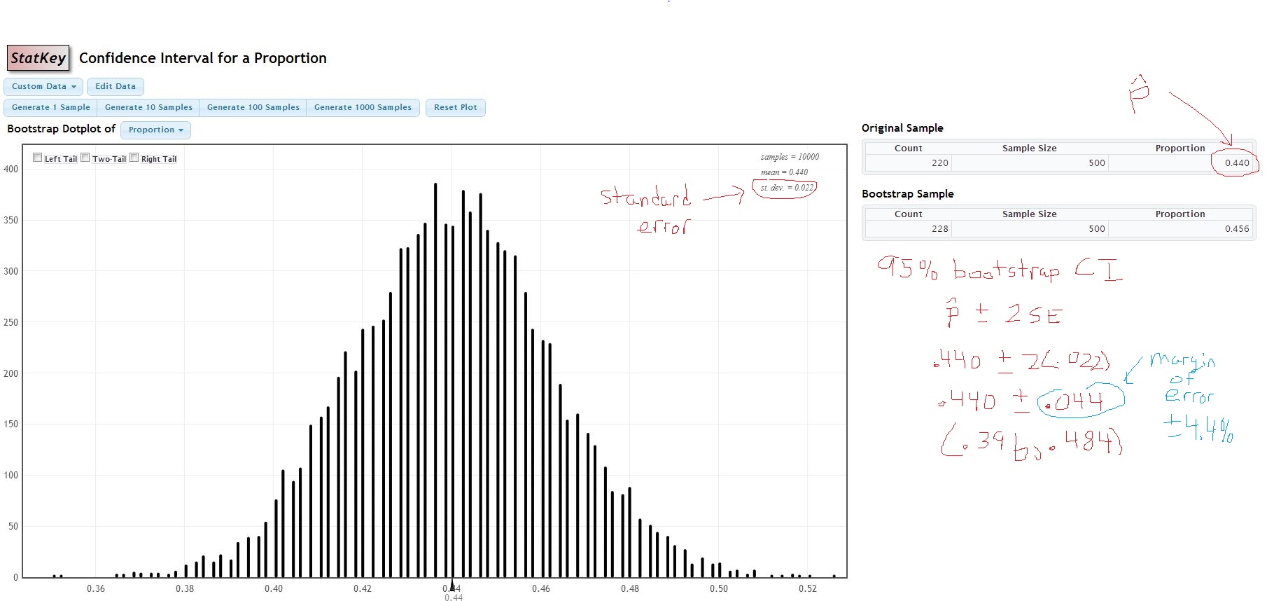
Go to http://www.lock5stat.com/statkey/index.html. Click on CI for Single Proportion and change the data from Mixed Nuts to Voter Sentiment. The Voter Sentiment example is similar to mine. Click on Edit Data and change count to 220 and sample size to 500 to match my example. We have an observed (real-life) data set with a count of \(X=220\) successes in a random sample of size \(n=500\), giving us a sample proportion of \(\hat{p}=\frac{220}{500}\).
Click on Generate One Sample. This will generate a single bootstrap sample. If you wanted to draw a single bootstrap sample physically, rather than computer simulation, you would need 500 balls, with 220 of them white (to represent our count of successes) and 500-220=280 of them black (to represent our count of failures). You, of course, could use different objects like cards, jelly beans, etc. We then draw a sample of size 500 (the size of our real-life observed sample) from our urn of 500 balls/cards/jelly beans/etc., but drawing WITH replacement.
When we do this, we will probably NOT get the exact same count and same sample proportion as in our real-life example. I happened to get \(X=210\) and \(\hat{p}=0.42\) with my first bootstrap sample.
Now, do this again. And again. And again. After a while, you’ll want to draw 10 or 100 or 1000 samples at once. Draw 10000 bootstrap samples. What do you notice about the shape of your sampling distribution?
When I drew 10000 samples, my screen looked like this:
BootstrapCI
As you see, the standard deviation of the sampling distribution (we call it standard error) is \(SE=0.022\), the margin of error is approximately twice this, or \(\pm 4.4%\), and the bootstrapped CI is virtually identical to the traditional CI. We’d see a larger difference when the sample size is small.
The standard error method of boostrapping a CI is called Method #2 in the book and in general is the orginal estimate of the statistic (call it \(\hat{\theta}\) plus/minus a critical value times the bootstrapped standard error (which is the standard deviation of all your bootstrap statistics).
In this example, we had an original proportion \(\hat{p}=\frac{220}{500}-0.44\), used \(z^* \approx 2\) for a roughly 95% interval, and \(B=10000\) bootstrap estimates \(\hat{p}^*\), where the standard error was \(SE=0.022\). Thus the interval was \(0.44 \pm 2(0.022)\).
The percentile method of constructing bootstrap intervals (called Method #1 in the book) does not utilize the standard error and thus does not assume that the sampling distribution is approximately normal, but does assume it is symmetric. We literally just take the middle 95% of values by taking the 2.5th and 97.5th percentiles, throwing away 5/2=2.5% on each end. To do this in StatKey, just check the Two-Tail box. If you want a confidence level other than 0.95, click and change that value.

BootstrapCI
The values on the two ends show up in red and the endpoints are indicated; in my simulation, about (0.398,0.484), which is very similar to what I obtain with the traditional formula or the bootstrapped standard error method.
Whether we construct CIs through the traditional frequentist formulas or via bootstrapping, they are still tricky to interpret. It is NOT correct to see ‘we are 95% sure that the true proportion is between 0.398 and 0.484’; instead, we realize that 95% of CIs drawn from random samples of our size will capture the true value of \(p\) and 5% are ‘unlucky’ and miss the true value of \(p\).
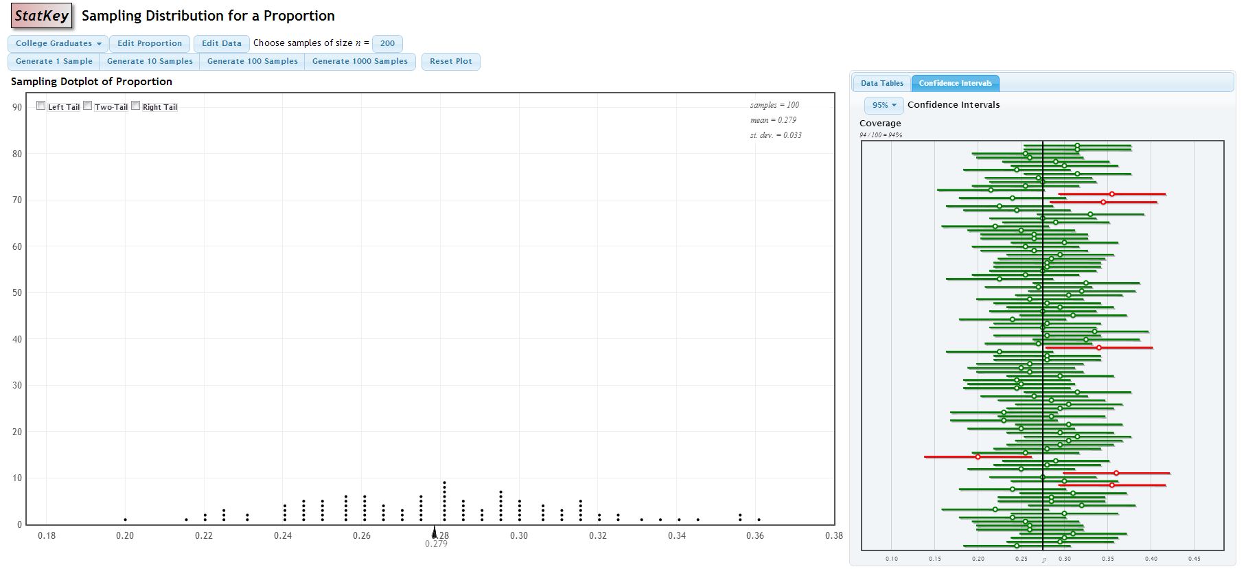
A nifty applet for showing this visually can be obtained in StatKey. Go back to the original StatKey page and click on Sampling Distributions: Proportion (right hand side). We’ll use their College Graduates example. This example is based on the fact that 27.5% of Americans are college graduates; in other words, we know that the parameter \(p=0.275\). Click on the Confidence Intervals tab on the right and Generate 100 Samples. Each of the bootstrap samples has a CI that is graphed; ones that included the true parameter \(p=0.275\) show up in green; ones that miss show up in red. Over the long run, about 5% should miss, so we expect about 5 red CIs.
BootstrapCI
I got 6 red CIs that ‘missed’ in my simulation.
4.3 The Bootstrapping Principle
The bootstrap is a flexible way to estimate parameters, particularly interval estimates, especially if either no theory exists for a CI formula or the assumptions for such a method are flawed.
The basics are that instead of the “leave-one-out” idea, we use a resampling idea, where we draw a sample WITH REPLACEMENT from the original sample. That is called a bootstrap sample, where some data points are sampled multiple times, with others not sample at all. We then compute the statistic of interest from that bootstrap sample. Then rinse-and-repeat \(B\) times (typically \(B=1000\) or more).
If we let \(\hat{\theta}\) be the value of the statistic computed from the original sample and \(X^{*b}\) be the \(b^{th}\) bootstrap sample drawn with replacement, then the \(b^{th}\) bootstrap sample statistic is \[\hat{\theta}^{*b}\]
Once we have this collection of \(B\) bootstrapped sample statistics \(\hat{\theta}^{*1}, \cdots, \hat{\theta}^{*B}\), (call this our bootstrap distribution) we have a variety of methods to compute a confidence interval or a hypothesis test that does not rely on classical statistical theory. We’ll just look at a few of these methods.
4.4 Bootstrapping a CI for a Mean
The process for constructing a bootstrap CI for a mean \(\mu\) using either the standard error or percentile method is very similar. Again, recall the traditional formula, which can be based on the normal distribution if the data is assumed to be normal, so \(X \sim N(\mu,\sigma^2)\) with a known standard deviation \(\sigma\)
\[\bar{x} \pm z^* \frac{\sigma}{\sqrt{n}}\]
or more realistically on the \(t\)-distribution when \(\sigma\) is an unknown nuisance parameter estimated by the sample standard deviation \(s\)
\[\bar{x} \pm t^* \frac{s}{\sqrt{n}}\]
Here \(\bar{x}\), the sample mean, is a statistic used to estimate the parameter \(\mu\), \(\frac{s}{\sqrt{n}}\) is the standard error for \(\bar{x}\), and \(t^*\) is a critical value from the \(t\)-distribution based on the degrees of freedom and the confidence interval that you desire. The TInterval function on the calculator is used for this calculation, using \(df=n-1\) or can be done with R with the MeanCI function from the DescTools package.
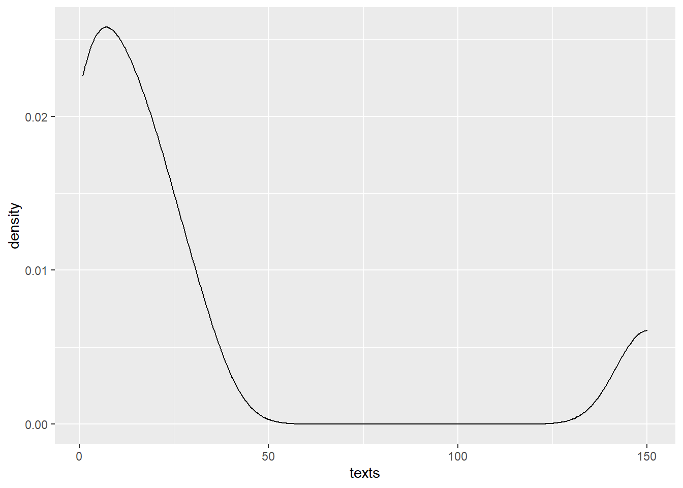
In class, we collected a random (?) sample of size \(n=8\) which consisted of the number of text message we had sent the previous day.
| Name | Texts |
|---|---|
| Chris | 1 |
| C.J. | 1 |
| Austin | 10 |
| Makayla | 4 |
| Kara | 19 |
| Ben | 30 |
| Adam | 17 |
| Jon | 150 |
We can see that the sample size is small and unlikely to be normally distributed, so reliance on the Central Limit Theorem to use the standard formula is not advised. Jon’s large value is clearly an outlier! I computed the 95% CI using the usual formula with the MeanCI function, but it’s probably not very accurate!
require(tidyverse)
require(mosaic)
require(DescTools)
name <- c("Chris","C.J.","Austin","Makayla","Kara",
          "Ben","Adam","Jon")
texts <- c(1,1,10,4,19,30,17,150)
texts.data <- tibble(name,texts)
favstats(~texts,data=texts.data)
## min Q1 median Q3 max mean sd n missing
## 1 3.25 13.5 21.75 150 29 49.91421 8 0## mean lwr.ci upr.ci
## 29.00000 -12.72933 70.72933
 We can enter this data into StatKey and obtain bootstrapping CIs using either the percentile or standard error methods.
Go to http://www.lock5stat.com/StatKey/ and pick CI for Single Mean, Median, Std. Dev.. Go to Edit Data and enter our sample of \(n=8\).
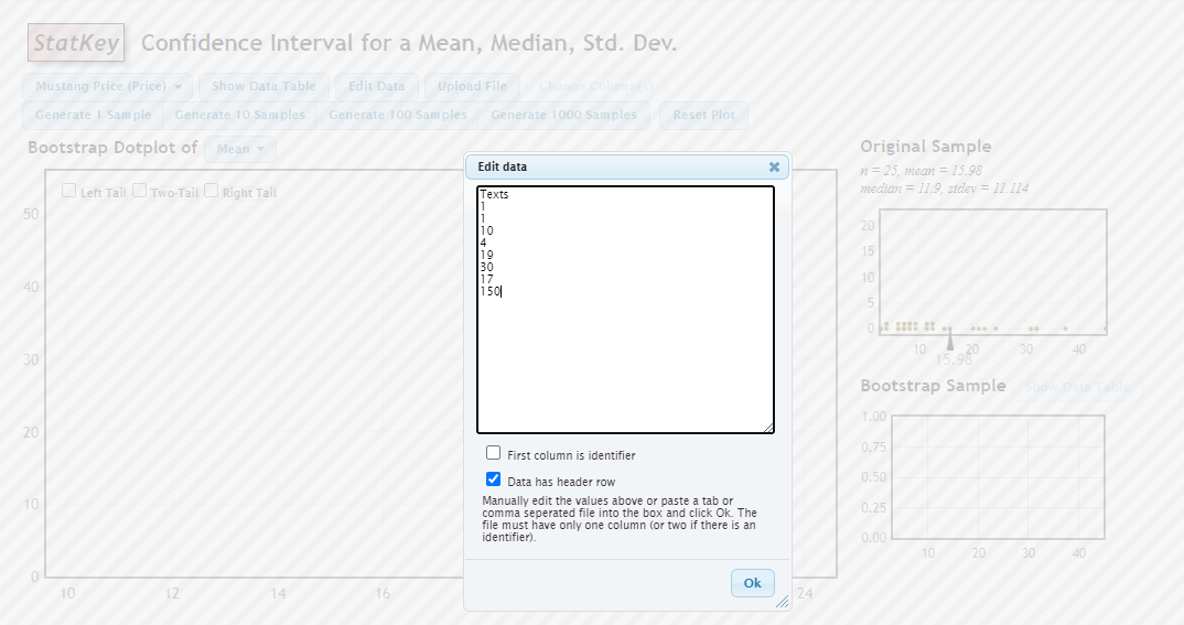
StatKey Edit Data
Now you can simulate a single bootstrap sample. We could do it “by hand” by selecting 8 random numbers WITH replacement between 1 and 8. If you have an eight-sided die, roll it 8 times and record the numbers. You could also use RandInt(1,8) on a TI-84 or the following R code.
## [1] 6 7 1 7 5 1 5 4In any single bootstrap sample, it is likely some individuals are sampled multiple times and others not at all. Here, person #1 (me), person #5 (Kara), and person #7 (Adam) were selected twice, persons #4 and #6 (Makayla & Ben) once, and persons #2, #3, and #8 (C.J., Austin, Jon) were not selected at all.
My first bootstrap statistic will be the mean. Generically these values will be \[\hat{\theta}^{*1},\hat{\theta}^{*2},\cdots,\hat{\theta}^{*B}\] if we are selecting \(B\) bootstrap samples.
In our case \[\bar{x}^{*1}=\frac{30+17+1+17+19+1+19+4}{8}=13.5\] which is less than the sample mean \(\bar{x}=29\) in the original sample. We didn’t sample Jon, with by far the largest value, in this particular bootstrap.
I generated \(B=1000\) bootstrap samples by pushing the Generate 1000 Samples button.
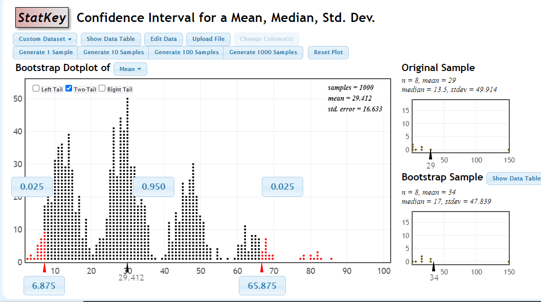
StatKey Bootstrap Mean
I checked the Two-Tail box inside the dotplot to get the 95% CI with the percentile method, which is \[(6.875,65.875)\] The red dots are the smallest 2.5% and largest 2.5% of the bootstrap estimates of the mean.
The standard error method yields the following as an approximate 95% CI, using \(\bar{x}=29\) (the estimate of the mean from the original data), \(z^* \approx 2\) and a bootstrap \(SE=16.633\).
\[29 \pm 2(16.633)\] \[ 29 \pm 33.266\] \[(-4.266,33.266)\] The answers from the traditional formula and the two basic bootstrapping methods differ quite a bit. Unfortunately, the basic bootstrapping methods assume that the bootstrapping distribution (as pictured in the dotplot) is symmetric (for the percentile method) and approximately normal, which are clearly not true.
Later, we’ll see more advanced bootstraps to use in this situation such as the bootstrap-t and the \(BCa\) bootstrap (bias corrected-accelerated).
We could compute the bias of our bootstrap. \[bias = \hat{\theta} - \bar{\theta^*}\] where \(\hat{\theta}\) is the estimate of the parameter using the original sample and \(\bar{\hat{\theta}}^*\) is the mean of the bootstrap statistics.
Here, we get \(bias=29-29.412=-0.412\).
4.5 Bootstrapping a CI for the Slope of a Regression Model
In this example, we are going to use bootstrapping rather than the standard formula to find a confidence interval for the slope of a regression model. The three methods in the book (percentile, standard error, and bootstrap-\(t\)) will be used.
In the bootstrap-\(t\) method, we do not assume that our bootstrap distribution is normal or near-normal and use a critical value from the standard normal or \(t\) distributions. Instead, we use bootstrapping to simulate our own \(t\)-table to find the critical values.
This is accomplished with the TSTAR function in the code below.
For each bootstrap sample in regression, we sample with replacement observations from the data set; here, each data point is a horse with a measurment for Height and Price. The regression model is fit for each bootstrap, and estimates of the slope (\(\hat{\beta_1}^*\)) and standard error of the slope are computed. Then the statistic \(T*\) is computed.
\[T^* = \frac{\hat{\theta}-\hat{\theta}^*}{SE_{\hat{\theta}^*}}\] Once we have computed \(B\) bootstraps, we find the \(\frac{\alpha}{2}\) and \(1-\frac{\alpha}{2}\) quantiles of our \(T^*\) distribution. These values serve as our critical values rather than getting them from standard tables. The book’s notation, assuming \(\alpha=0.05\) for a 95% confidence interval, is \(qt_{0.025}\) and \(qt_{0.975}\).
The lower limit of the bootstrap-\(t\) interval is: \[\hat{\theta}-qt_{0.975} \cdot SE\] The upper limit of the bootstrap-\(t\) interval is: \[\hat{\theta}-qt{0.025}\cdot SE\]
where \(SE\) is the standard error of the statistic (here, the slope) in the original sample.
The code below computes four different confidence intervals for the slope (traditional formula, percentile bootstrap, standard error bootstrap, bootstrap-\(t\)), along with the bootstrap bias.
# percentile, standard error, bootstrap-t for slope of a regression line
require(Stat2Data)
data(HorsePrices)
HorsePrices <- HorsePrices %>% na.omit

ggplot(HorsePrices,aes(x=Height,y=Price)) +
  geom_point() + geom_smooth(method="lm")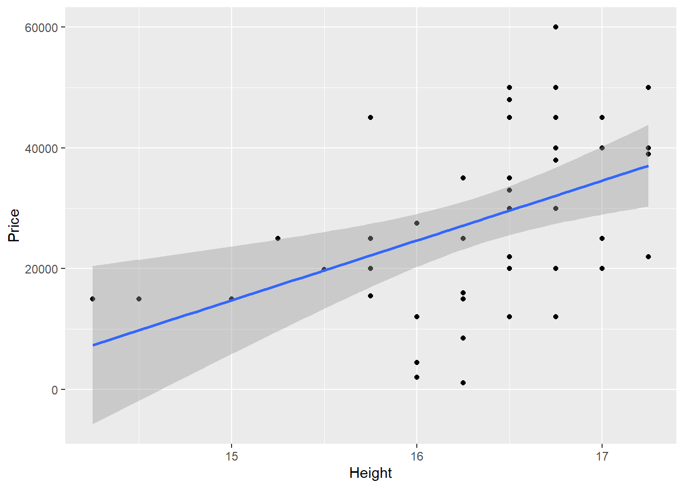
##
## Call:
## lm(formula = Price ~ Height, data = HorsePrices)
##
## Residuals:
##    Min     1Q Median     3Q    Max
## -26067 -11167   1928   7833  27880
##
## Coefficients:
##             Estimate Std. Error t value Pr(>|t|)
## (Intercept)  -133791      48817  -2.741  0.00876 **
## Height          9905       2987   3.316  0.00181 **
## ---
## Signif. codes:  0 '***' 0.001 '**' 0.01 '*' 0.05 '.' 0.1 ' ' 1
##
## Residual standard error: 13360 on 45 degrees of freedom
## Multiple R-squared:  0.1964,	Adjusted R-squared:  0.1785
## F-statistic: 11 on 1 and 45 DF, p-value: 0.001812## 2.5 % 97.5 %
## (Intercept) -232113.754 -35469.10
## Height 3888.903 15921.38## Height
## 9905.143## [1] 2987.056TSTAR <- function(x){
regstar <- lm(Price~Height,data=resample(x))
est.star <- coefficients(regstar)[2]
SE.star <- coefficients(summary(regstar))[2,2]
tstar <- (est.star-est)/ SE.star
stats <- c(est.star,SE.star,tstar)
names(stats) <- c("est.star","SE.star","tstar")
return(stats)
}
b <- 1000
boot.reg <- do(b)*TSTAR(HorsePrices)
t.stars <- boot.reg$tstar
# visualize the t.stars
ggplot(tibble(t.stars),aes(x=t.stars)) + geom_density()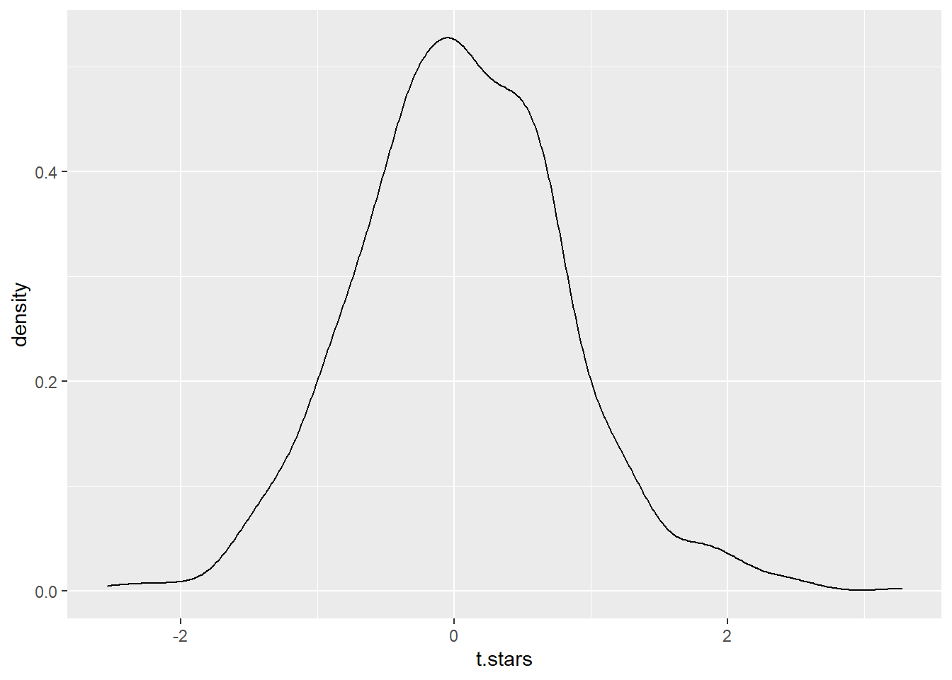
# visualize the bootstrap distribution
# ideally this would be symmetric rather than skewed
# since it is skewed, I would want a more advanced bootstrapping method
# like bootstrap-t or BCa (bias-corrected and accelerated)

ggplot(boot.reg,aes(x=est.star)) +
  geom_histogram(bins=20,fill="lightblue",color="blue")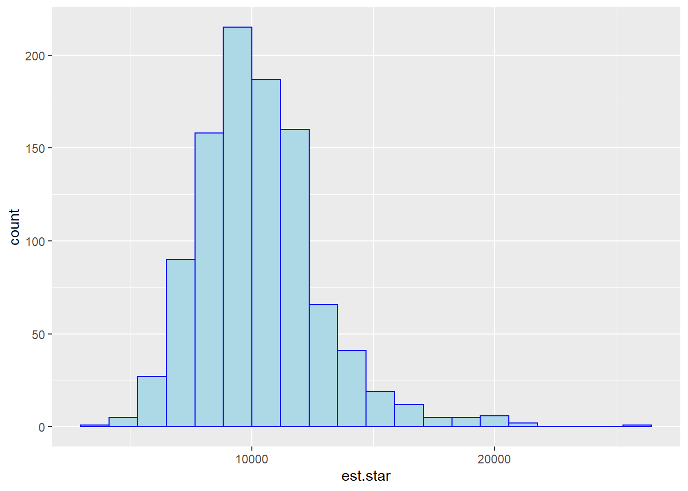
ggplot(boot.reg,aes(x=est.star)) +
  geom_dotplot(dotsize=0.05,binwidth=1000,breaks=c(0,5000,10000,15000,20000))
# percentile bootstrap method
alpha <- 0.05 # for 95% confidence
quantile(x=boot.reg$est.star,probs=c(alpha/2,1-alpha/2),data=boot.reg)
## 2.5% 97.5%
## 6294.237 16318.607# standard error bootstrap method
# original estimate plus/minus critical value times standard error of bootstrap
SE.boot <- sd(boot.reg$est.star)
est + c(-1,1)*qnorm(p=1-alpha/2)*SE.boot## [1] 4945.97 14864.32# bootstrap-t method
qt025 <- quantile(t.stars,probs=0.025)
qt975 <- quantile(t.stars,probs=0.975)
boot.t.lower <- est - qt975*SE
boot.t.upper <- est - qt025*SE
boot.t.CI <- c(boot.t.lower,boot.t.upper)
boot.t.CI## Height Height
## 4652.762 14101.704## Height
## -401.10214.6 Bootstrapping a CI for Interquartile Range
Here, we take the mpg variable mtcars data set, the gas mileage (in miles per gallon) for \(n=32\) cars. The parameter of interest is the interquartile range, \[IQR=Q_3-Q_1\] You probably never learned a formula for the confidence interval of the IQR.
We compute the IQR for the data set and refer to this statistic as est or \(\hat{\theta}\). \(B=1000\) bootstrap samples were generated and the IQR was computed for each bootstrap.
require(mosaic)
require(tidyverse)
# percentile, standard error, BCa methods for IQR
data(mtcars)
summary(mtcars)
## mpg cyl disp hp
## Min. :10.40 Min. :4.000 Min. : 71.1 Min. : 52.0
## 1st Qu.:15.43 1st Qu.:4.000 1st Qu.:120.8 1st Qu.: 96.5
## Median :19.20 Median :6.000 Median :196.3 Median :123.0
## Mean :20.09 Mean :6.188 Mean :230.7 Mean :146.7
## 3rd Qu.:22.80 3rd Qu.:8.000 3rd Qu.:326.0 3rd Qu.:180.0
## Max. :33.90 Max. :8.000 Max. :472.0 Max. :335.0
## drat wt qsec vs
## Min. :2.760 Min. :1.513 Min. :14.50 Min. :0.0000
## 1st Qu.:3.080 1st Qu.:2.581 1st Qu.:16.89 1st Qu.:0.0000
## Median :3.695 Median :3.325 Median :17.71 Median :0.0000
## Mean :3.597 Mean :3.217 Mean :17.85 Mean :0.4375
## 3rd Qu.:3.920 3rd Qu.:3.610 3rd Qu.:18.90 3rd Qu.:1.0000
## Max. :4.930 Max. :5.424 Max. :22.90 Max. :1.0000
## am gear carb
## Min. :0.0000 Min. :3.000 Min. :1.000
## 1st Qu.:0.0000 1st Qu.:3.000 1st Qu.:2.000
## Median :0.0000 Median :4.000 Median :2.000
## Mean :0.4062 Mean :3.688 Mean :2.812
## 3rd Qu.:1.0000 3rd Qu.:4.000 3rd Qu.:4.000
## Max. :1.0000 Max. :5.000 Max. :8.000
# do B bootstrap samples
theta.hat <- IQR(mtcars$mpg) # 22.80 - 15.43 = 7.37
set.seed(2502852) # to repeat my results
B <- 1000
boot.IQR <- do(B)*IQR(resample(mtcars$mpg,replace=TRUE))
boot.IQR <- data.frame(boot.IQR)
head(boot.IQR)
## IQR
## 1 7.600
## 2 5.150
## 3 6.000
## 4 6.250
## 5 5.350
## 6 8.375We’ll visualize the bootstrap distribution with both a histogram and a dotplot. Experiment with the number of bins in the histogram, or the dotsize/breaks in the dotplot.
The percentile and standard error methods are used to compute 95% confidence intervals for the interquartile range of the mpg variable.
# visualize the bootstrap distribution
# ideally this would be symmetric rather than skewed
# since it is skewed, I would want a more advanced bootstrapping method
# like bootstrap-t or BCa (bias-corrected and accelerated)

ggplot(boot.IQR,aes(x=IQR)) +
  geom_histogram(bins=20,fill="lightblue",color="blue")
ggplot(boot.IQR,aes(x=IQR,y=1)) + geom_dotplot(dotsize=0.5,binwidth=0.2) + theme(axis.text.y=element_blank()) + scale_x_continuous(breaks=c(4,6,8,10,12,14,16))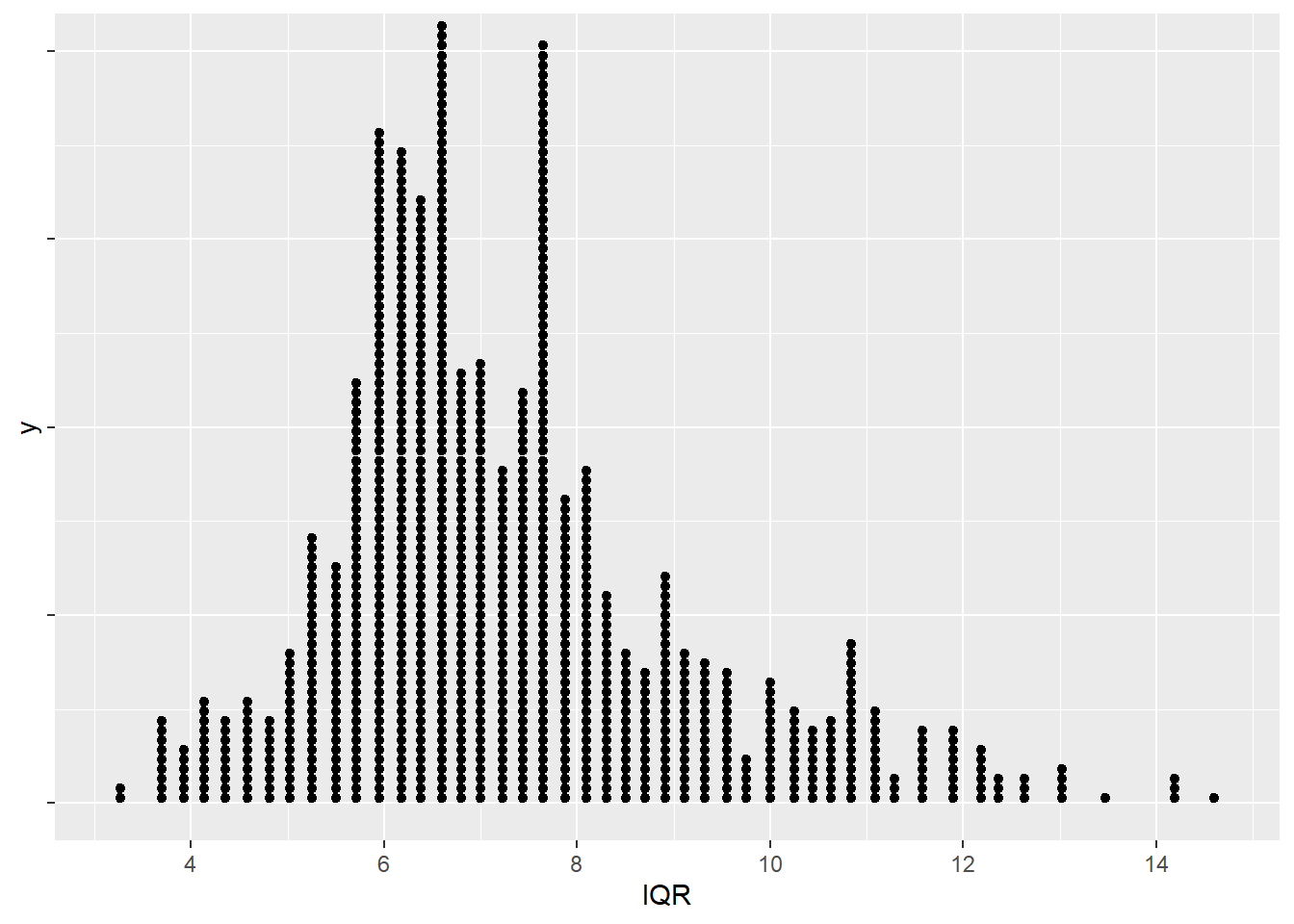
# percentile bootstrap
alpha <- 0.05 # for 95% confidence
quantile(x=boot.IQR$IQR,probs=c(alpha/2,1-alpha/2),data=boot.IQR)
## 2.5% 97.5%
## 4.149375 11.875625# standard error bootstrap
# original estimate plus/minus critical value times standard error of bootstrap
SE.boot <- sd(boot.IQR$IQR)
theta.hat + c(-1,1)*qnorm(p=1-alpha/2)*SE.boot## [1] 3.761334 10.988666Since the bootstrap distribution is skewed, the results of the percentile or standard error intervals are questionable. I don’t know what to use as the standard error \(SE\) for the \(IQR\), so I can’t use the bootstrap-\(t\).
The \(BCa\) bootstrap is an option here, where the bootstrap is correction for bias (\(BC\)) and “accelerated” (\(a\)). “Accelerated” means that we also have a correction for skewness.
The mathematical derivations are not given and this method is certainly not as intuitive as the other methods of bootstrapping (and is not in our textbook).
First, compute the bias correction. We find the proportion \(p_{less}\) of the bootstrap statistics \(\hat{\theta}^*\) that less than the original estimate \(\hat{\theta}\). Then compute the inverse CDF of the standard normal distribution (i.e. find a \(z\)-score) of \(p_{less}\). If exactly half of the bootstrap estimates are less than the original estimate, then this estimate \(z_0\) will be equal to zero, which means there is no bias correction.
\[p_{less}=\frac{\text{# of }\hat{\theta}^* < \hat{\theta}}{B}\]
\[z_0 = \Phi^{-1}(p_{less})\]
## [1] 0.579## [1] 0.1993359The correction for skewness (“acceleration”) is more difficult. We compute the \(n\) jackknife (leave-one-out) estimates of the statistic, \(\hat{\theta}_{(-i)}\). Then find the mean of the jackknife estimates, call it \[\bar{J}=\frac{\sum_{i=1}^n \hat{\theta}_{(-i)}}{n}\]
The acceleration correction \(\hat{a}\) is \[a=\frac{(\sum_{i=1}^n \bar{J}-\hat{\theta}_{(-i)})^3}{6[(\sum_{i=1}^n \bar{J}-\hat{\theta}_{(-i)})^2]^{3/2}}\]
x <- mtcars$mpg
n <- nrow(mtcars)
IQR.jack <- numeric(n)
for (i in 1:n){
  temp <- x[-i]
  # leave that one out
  IQR.jack[i] <- IQR(temp)
}
IQR.jack
## [1] 7.45 7.45 6.80 7.45 7.45 7.45 7.15 6.80 6.80 7.45 7.45 7.45 7.45 7.15 7.15
## [16] 7.15 7.15 6.80 6.80 6.80 7.45 7.30 7.15 7.15 7.45 6.80 6.80 6.80 7.45 7.45
## [31] 7.15 7.45## [1] 7.1875## [1] 0.01254536The BCa interval is computed by calculating \[z_L = z_0 + \Phi^{-1}(\alpha/2)\] \[z_U = z_0 + \Phi^{-1}(1-\alpha/2)\] \[\alpha_1 = \Phi(z_0 + \frac{z_L}{1-\hat{a}z_L})\] \[\alpha_2 = \Phi(z_0 + \frac{z_U}{1-\hat{a}z_U})\] The BCa interval are the \(\alpha_1\) and \(\alpha_2\) quantiles of the \(B\) bootstrap estimates.
# compute the 100(1-alpha)% BCa interval
zL <- z0 + qnorm(p=alpha/2)
# this is z0-1.96 for 95%
alpha1 <- pnorm(z0+zL/(1-a.hat*zL))
# this is P(Z < z0+zL/(1-a.hat*zL))
zU <- z0 + qnorm(p=1-alpha/2)
alpha2 <- pnorm(z0+zU/(1-a.hat*zU))
BCa.CI <- quantile(probs=c(alpha1,alpha2),x=boot.IQR$IQR)
BCa.CI
## 6.384879% 99.22132%
## 5.083871 12.9610504.7 Permutation Test
Fisher’s classic Zea Mays problem (from Darwin’s data) was used to illustrate paired samples t-test and the “permutation test” within each pair, there is one corn seedling that is cross-fertilized
and the other corn seedling is self-fertilized. The response is final height (in inches) of the seedling, where diff is cross - self.
In a permutation test, we compute all possible permutations of the test statistic in question, which in a paired samples problem is diff. For a sample of size \(n\), there are \(2^n\) possible permutations. In the Zea Mays problem, this is \(2^{15}=32768\), which gives us some idea why the theory of permutation tests from the 1930s did not catch on until computers were available.
The p-value of a permutation test is literally how unusual our observed test statistic is from the distribution of all possible test statistics. We don’t rely on a probability distribution such as the normal, \(t\), \(F\), or \(\chi^2\).
If the number of permutations is too large, then a large number of such values are simulated.
##    pair pot  cross   self   diff
## 1     1   1 23.500 17.375  6.125
## 2     2   1 12.000 20.375 -8.375
## 3     3   1 21.000 20.000  1.000
## 4     4   2 22.000 20.000  2.000
## 5     5   2 19.125 18.375  0.750
## 6     6   2 21.500 18.625  2.875
## 7     7   3 22.125 18.625  3.500
## 8     8   3 20.375 15.250  5.125
## 9     9   3 18.250 16.500  1.750
## 10   10   3 21.625 18.000  3.625
## 11   11   3 23.250 16.250  7.000
## 12   12   4 21.000 18.000  3.000
## 13   13   4 22.125 12.750  9.375
## 14   14   4 23.000 15.500  7.500
## 15   15   4 12.000 18.000 -6.000
## [1] 2.616667##
## One Sample t-test
##
## data: diff
## t = 2.148, df = 14, p-value = 0.0497
## alternative hypothesis: true mean is not equal to 0
## 95 percent confidence interval:
## 0.003899165 5.229434169
## sample estimates:
## mean of x
## 2.616667# p-value just under alpha=0.05 for 2 sided t-test but assumptions are questionable
# we will do a "tactile simulation" of a random permutation of the difference
# via coin-flipping
# heads = cross - self, tails = self - cross (i.e. if tails, multiply diff by -1)
coin <- c(1,-1) #heads is +1, tails is -1
toss <- sample(size=15,x=coin,replace=TRUE)
toss## [1] 1 -1 1 -1 -1 -1 -1 -1 1 1 -1 1 -1 -1 1permutation.sample1 <- ZeaMays$diff * toss
mean(permutation.sample1) #this is the mean Dbar of your permuation## [1] -1.35# There are 2^n possible permutations, can all be computed if n is small enough
# So we construct a sampling distribution of all permutations rather than
# assuming the sampling distribution of the t-statistic is a t-distribution
# Fancy code someone else wrote to do this (you won't need to do this)
# came from help(ZeaMays)
# complete permutation distribution of diff, for all 2^15 ways of assigning
# one value to cross and the other to self (thx: Bert Gunter)
N <- nrow(ZeaMays)
allmeans <- as.matrix(expand.grid(as.data.frame(
matrix(rep(c(-1,1),N), nr =2)))) %*% abs(ZeaMays$diff) / N
# upper-tail p-value
sum(allmeans > mean(ZeaMays$diff)) / 2^N## [1] 0.02548218## [1] 0.05096436# for the exact 2-sided permutation test, p-value just above alpha=0.05
ggplot(tibble(allmeans),aes(x=allmeans)) +
geom_histogram(fill="lightblue",color="blue",bins=64) +
geom_vline(xintercept=c(-1,1)*mean(ZeaMays$diff),color="red",linetype="dashed")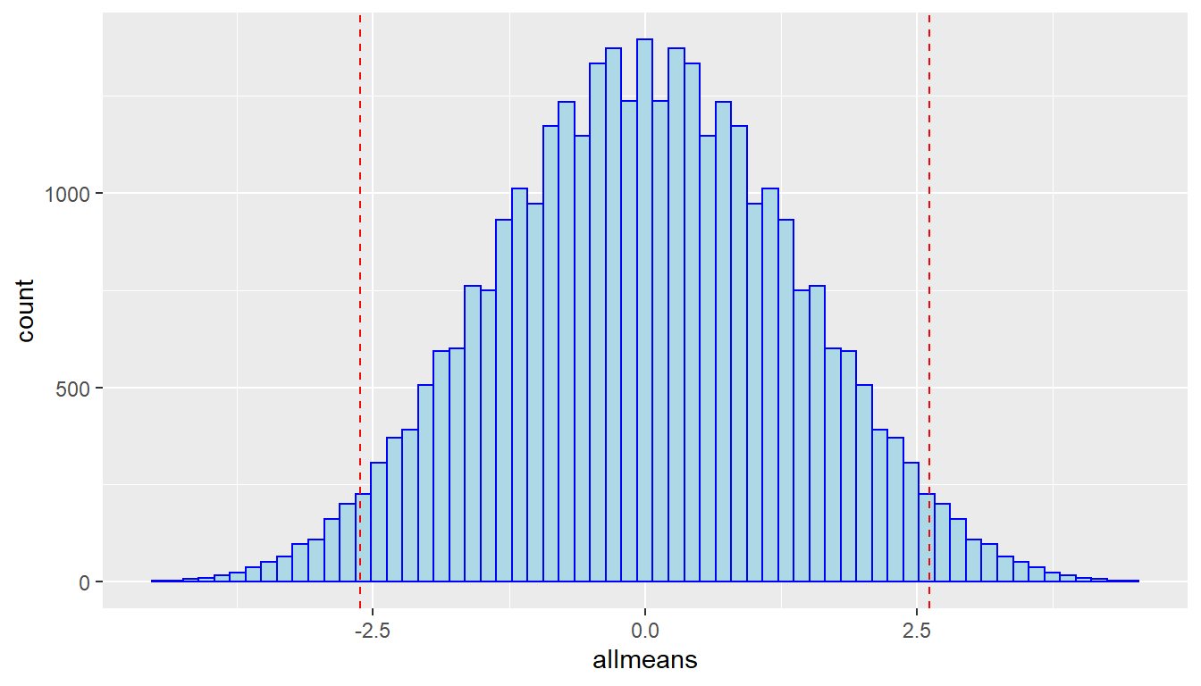
4.8 Randomization Test
Test of means from two groups (sleep and memory)
Using the reallocate or “shuffle” method, all cases in the samples are combined and then randomly assigned to the two groups with the same sample sizes as the original samples. This is done without replacement. The mean (or other test statistic of interest) of each reallocated or “shuffled” sample is recorded.
In an experiment on memory (Mednicj et al, 2008), students were given lists of 24 words to memorize. After hearing the words they were assigned at random to different groups. One group of 12 students took a nap for 1.5 hours while a second group of 12 students stayed awake and was given a caffeine pill. The results below display the number of Words each participant was able to recall after the break. Test whether the data indicate a difference in mean number of words recalled between the two treatments, Group.
## Caffeine    Sleep
## 12.25 15.25## Sleep
## 3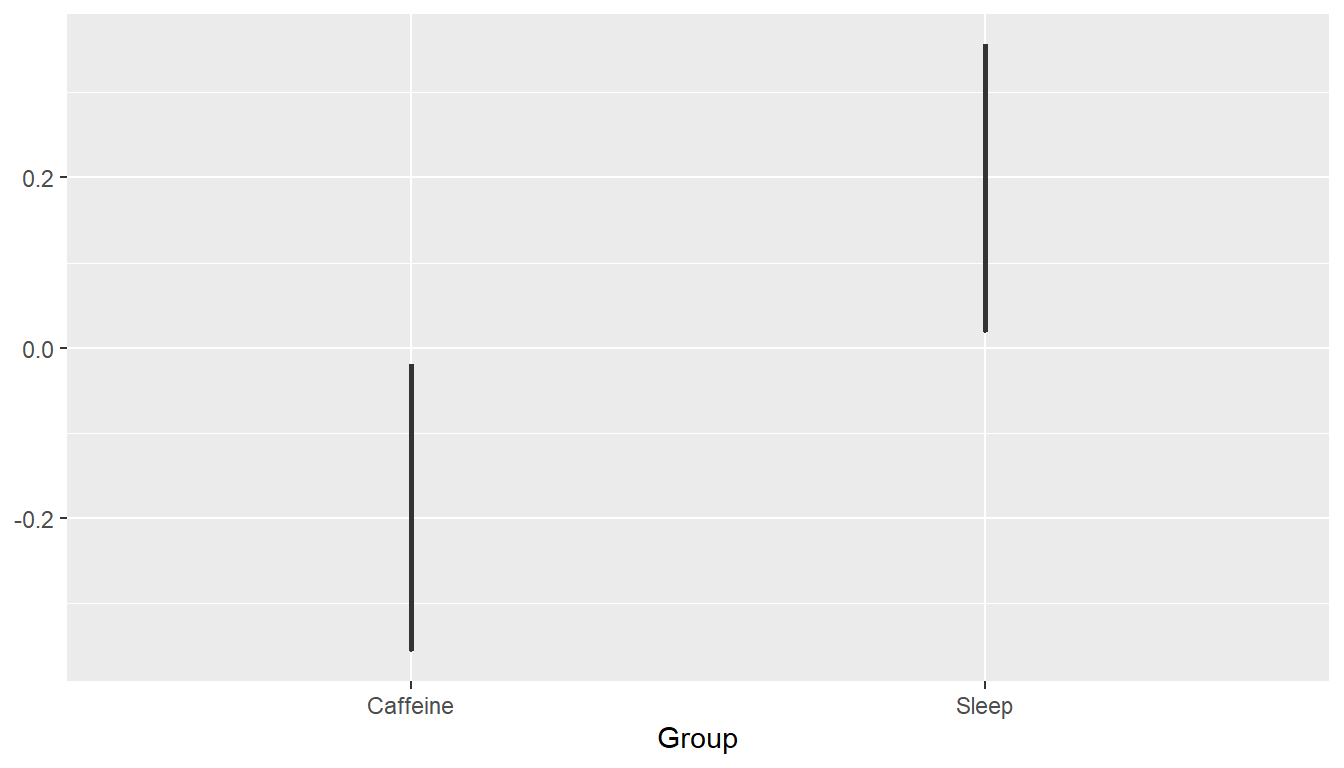
#To implement the null hypothesis, shuffle the Group with respect to the outcome, Words:
diff(mean(Words ~ shuffle(Group), data=SleepCaffeine)) #one permutation or "shuffle"
## Sleep
## 0.8333333## Sleep
## 2.333333# To get the distribution under the null hypothesis, we carry out many trials:
set.seed(93619)
Sleep.null <- do(1000) * diff(mean(Words ~ shuffle(Group), data=SleepCaffeine))
ggplot(Sleep.null,aes(x=Sleep,fill=(Sleep<=obs))) +
geom_histogram(color="black")
#onesided p-value, alternative is that Sleep > Caffeine Pill
pvalue <- sum(Sleep.null>obs)/1000
pvalue
## [1] 0.0164.9 Bootstrapping and Randomization Testing for Correlation/Regression
Bootstrapping a correlation, testing for significance of the correlation
The data on Mustang prices contains the number of miles each car had been driven (in thousands). Find a 95% confidence interval for the correlation between price and mileage. You probably don’t know the formula for a confidence interval of a correlation (although one does exist, albeit requiring the Fisher’s z transformation).
With the SATGPA data, we’ll do a hypothesis test of the null hypothesis that \(\rho=0\) between a student’s GPA and verbal SAT score. We could have test for significance of the slope of the regression line, or done a t-test for the correlation.
##   Age Miles Price
## 1   6   8.5  32.0
## 2   7  33.0  45.0
## 3   9  82.8  11.9
## 4   2   7.0  24.8
## 5   3  23.0  22.0
## 6 15 111.0 10.0## Age Miles Price orig.id
## 22 13 72.7 8.0 22
## 6 15 111.0 10.0 6
## 17 6 71.2 16.0 17
## 21 10 86.4 9.7 21
## 2 7 33.0 45.0 2
## 23 13 71.8 11.8 23
## 1 6 8.5 32.0 1
## 19 12 117.4 7.0 19
## 4 2 7.0 24.8 4
## 2.1 7 33.0 45.0 2
## 18 1 26.4 21.0 18
## 20 14 102.0 8.2 20
## 10 1 1.1 37.9 10
## 10.1 1 1.1 37.9 10
## 6.1 15 111.0 10.0 6
## 7 10 136.2 5.0 7
## 16 9 61.9 7.0 16
## 22.1 13 72.7 8.0 22
## 18.1 1 26.4 21.0 18
## 13 8 100.8 9.0 13
## 6.2 15 111.0 10.0 6
## 19.1 12 117.4 7.0 19
## 13.1 8 100.8 9.0 13
## 8 9 78.2 9.0 8
## 2.2 7 33.0 45.0 2## [1] -0.8246164## -0.825
Mustangs.cor.boot <- do(1000) * cor(Price~Miles, data=resample(MustangPrice))
mean(~cor,data=Mustangs.cor.boot) #mean of bootstrap dist## [1] -0.8364193## [1] -0.01180285## [1] 0.05679392## [1] -0.9477354 -0.7251032## 2.5% 97.5%
## -0.9321434 -0.7234653## name lower upper level method estimate margin.of.error
## 1 cor -0.9321434 -0.7234653 0.95 percentile -0.8246164 NA
## 2 cor -0.9477333 -0.7251052 0.95 stderr -0.8246164 0.111314
# could do a fancier interval like bootstrap-t or BCa

# randomization test for correlation between GPA and VerbalSAT
#we will "scramble" the GPAs and randomly assign to the n=24 students

require(Stat2Data)
data(SATGPA)

obs.cor <- cor(GPA~VerbalSAT,data=SATGPA) # r = 0.244
# is this signifciantly different from zero?
set.seed(395296)
rand.cors <- do(1000)*cor(shuffle(GPA)~VerbalSAT,data=SATGPA)

rand.pvalue <- sum(abs(rand.cors)>=abs(obs.cor))/1000
rand.pvalue
## [1] 0.254##
## Call:
## lm(formula = GPA ~ VerbalSAT, data = SATGPA)
##
## Residuals:
## Min 1Q Median 3Q Max
## -0.62002 -0.25932 0.03885 0.20502 0.51621
##
## Coefficients:
## Estimate Std. Error t value Pr(>|t|)
## (Intercept) 2.6042036 0.4377919 5.948 0.0000055 ***
## VerbalSAT 0.0009056 0.0007659 1.182 0.25
## ---
## Signif. codes: 0 '***' 0.001 '**' 0.01 '*' 0.05 '.' 0.1 ' ' 1
##
## Residual standard error: 0.3154 on 22 degrees of freedom
## Multiple R-squared: 0.05976, Adjusted R-squared: 0.01702
## F-statistic: 1.398 on 1 and 22 DF, p-value: 0.2496## VerbalSAT
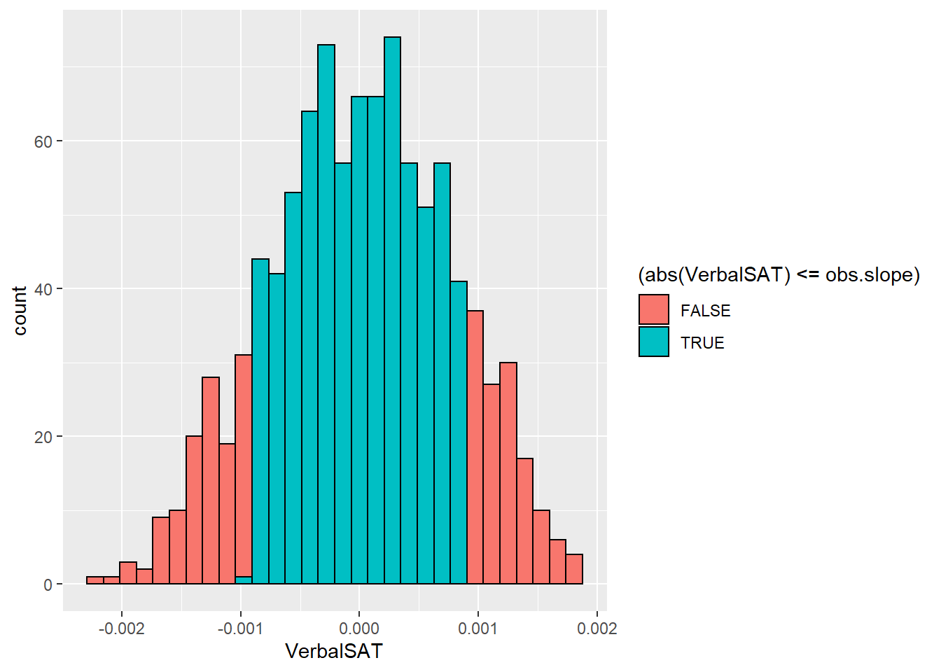
## 0.0009056089set.seed(395296)
rand.slopes <- do(1000)*lm(shuffle(GPA)~VerbalSAT,data=SATGPA)
rand.pvalu <- sum(abs(rand.slopes$VerbalSAT)>=abs(0.0009056))/1000
rand.pvalu## [1] 0.254ggplot(rand.slopes,aes(x=VerbalSAT,fill=(abs(VerbalSAT)<=obs.slope))) +
geom_histogram(color="black")