Chapter 7 ANOVA with Interaction

7.1 The Interactive Two-Way ANOVA Model

The model below includes two fixed-effects factors, an interaction term between the factors, and assumes a balanced design with $n>1$ replicates per treatment combination.

$Y_{ijk} = \mu + \alpha_i + \beta_j + \gamma_{ij} + \epsilon_{ijk}$

$i=1,2,\cdots,r$ , where $r$ is the number of levels of Factor A (the “row” factor)

$j=1,2,\cdots,c$ , where $c$ is the number of levels of Factor B (the “column” factor)

$k=1,2,\cdots,n_{ij}$ , where $n_{ij}$ is the number of replicates in cell $(i,j)$ (i.e. the combination of Factors A and B) and we’ll assume all $n_{ij}=n>1$ (same number in each cell)

$Y_{ijk}$ is the value of the response variable for the $k^{th}$ replicate with level $i$ of Factor A and level $j$ of Factor B.

The parameters of the model are:

$\mu$ : The overall mean response. We have 1 $\mu$ parameter.

$\alpha_i$ : The treatment effect of Factor A. We have $r$ $\alpha_i$ parameters.

$\beta_j$ : The treatment effect of Factor B. We have $c$ $\beta_j$ parameters.

$\gamma_{ij}$ (or $\alpha \beta_{ij}$ ): The interaction between Factors A and B. We have $r \times c$ $\gamma_{ij}$ parameters.

Note that $\gamma_{ij} = \mu_{ij} - \mu_{i.} - \mu_{.j} + \mu_{..}$ .

The errors are $\epsilon_{ijk} \sim N(0, \sigma^2)$ . With a balanced design, then $\sum \alpha_i =0$ , $\sum \beta_j =0$ and $\sum \gamma_{ij}=0$ .

7.2 Sums of Squares

The “fun” (???) formulas for sums of squares are given:

$\text{Sum of Squares Total:} \: \: SST = \sum_{i=1}^r \sum_{j=1}^c \sum_{k=1}^{n} (Y_{ijk}-\bar{Y}_{...})^2$

$\text{Sum of Squares Factor A(Row):} \: \: SSA = cn \sum_{i=1}^r (\bar{Y}_{i..}-\bar{Y}_{...})^2$

$\text{Sum of Squares Factor B(COlumn):} \: \: SSB = rn \sum_{j=1}^c (\bar{Y}_{.j.}-\bar{Y}_{...})^2$

$\text{Sum of Squares Interaction (AB):} \: \: SSAB = n \sum_{i=1}^r \sum_{j=1}^c (\bar{Y_{ij.}}-\bar{Y}_{i..}-\bar{Y}_{.j.}+\bar{Y}_{...})^2$ $\text{Sum of Squares Error:} \: \: SSE = \sum_{i=1}^r \sum_{j=1}^c \sum_{k=1}^n (Y_{ijk}-\bar{Y}_{ij.})^2$ $SSTotal = SSA + SSB + SSAB + SSE$

Did you puke yet?

7.3 ANOVA Table

We will have $r-1$ and $c-1$ degrees of freedom for the Factors A and B, respectively. The interaction degrees of freedom are $(r-1) \times (c-1)$ and the error degrees of freedom are $rc(n-1)$ . Notice that when $n=1$ there are zero degrees of freedom left for error, which is why we were forced to assume no interaction for the randomized block designs with $n=1$ .

Source	$df$	$SS$	$MS$	$F$	$p$ -value
Factor A (Row)	$r-1$	$SSA$	$MSA$	$MSA/MSE$	$F(A) \sim F(r-1,rc(n-1))$ df
Factor B (Column)	$c-1$	$SSB$	$MSB$	$MSB/MSE$	$F(B) \sim F(c-1,rc(n-1))$ df
Interaction	$(r-1)(c-1)$	$SSAB$	$MSAB$	$MSB/MSE$	$F(AB) \sim F((r-1)(c-1),rc(n-1))$
Error	$rc(n-1)$	$SSE$	$MSE$
Total	$rcn-1$	$SSY$

There are three different $F$ tests of interest. You should actually focus on the test of the interaction $F(AB)$ first, as if it is significant all of the interpretations will be based the existence of such an interaction.

Interaction: $F(AB)$ with $df=(r-1)(c-1),rc(n-1)$ , $H_O: \gamma_{ij}=0 \: \: \forall i,j$
Factor A: $F(A)$ with $df=r-1,rc(n-1)$ , $H_O: \alpha_i=0 \: \: \forall i$
Factor B: $F(B)$ with $df=c-1,rc(n-1)$ , $H_O: \beta_j=0 \: \: \forall j$

The latter two tests are referred to as “main effects”.

7.4 Interactions (What Are They?)

In ANOVA, an interaction is defined as when the difference in the means of the response between the levels of one factor is NOT the same across all levels of another factor.

In this section, I will have two levels of Factor A (the row variable) called $A1$ and $A2$ and two levels of Factor B (the column variable) called $B1$ and $B2$ , and a continuous response variable $Y$ . If you want a concrete example, think of Factor $A$ as being two different kinds of seed a farmer could plant, Factor $B$ as being two different types of fertilizer the farmer could use, and the response $Y$ as the yield of the crop, that the farmer wants to maximize. I have simulated data to represent various situations that could come up when conducting a two-way ANOVA.

First, let look at situations with no interaction, with both the main effects for $A$ and $B$ significant. The profiles will be parallel (or close to parallel). The points being plotted are the means of the treatment combinations.

## Analysis of Variance Table
## 
## Response: Y
##           Df Sum Sq Mean Sq  F value Pr(>F)    
## A          1 509.86  509.86 440.6372 <2e-16 ***
## B          1 466.94  466.94 403.5471 <2e-16 ***
## A:B        1   1.60    1.60   1.3835 0.2432    
## Residuals 76  87.94    1.16                    
## ---
## Signif. codes:  0 '***' 0.001 '**' 0.01 '*' 0.05 '.' 0.1 ' ' 1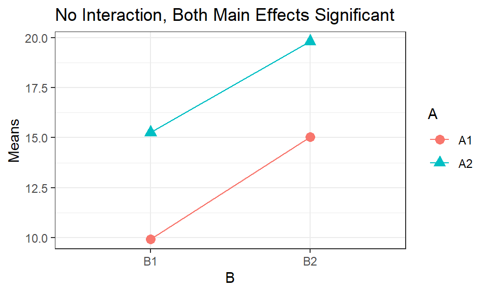

In this example, the farmer’s yield will be significantly higher using $A2$ and $B2$ .

Here are similar examples: one with only Factor A significant, another with only Factor B significant, and the final with no significant effects (where the profiles are essentially coincident).

## Analysis of Variance Table
## 
## Response: Y
##           Df  Sum Sq Mean Sq  F value Pr(>F)    
## A          1 180.850 180.850 199.4095 <2e-16 ***
## B          1   0.293   0.293   0.3227 0.5717    
## A:B        1   0.052   0.052   0.0570 0.8120    
## Residuals 76  68.926   0.907                    
## ---
## Signif. codes:  0 '***' 0.001 '**' 0.01 '*' 0.05 '.' 0.1 ' ' 1

In this example, the farmer’s yield will be significantly higher with $A2$ . There is no significant difference between $B1$ and $B2$ , so other considerations like price, environmental impact, etc. might be used to decide.

## Analysis of Variance Table
## 
## Response: Y
##           Df  Sum Sq Mean Sq  F value Pr(>F)    
## A          1   0.592   0.592   0.6500 0.4226    
## B          1 116.586 116.586 128.1173 <2e-16 ***
## A:B        1   0.101   0.101   0.1108 0.7401    
## Residuals 76  69.159   0.910                    
## ---
## Signif. codes:  0 '***' 0.001 '**' 0.01 '*' 0.05 '.' 0.1 ' ' 1

In this example, the farmer’s yield will be significantly higher with $B2$ . There is no significant difference between $A1$ and $A2$ , so again other considerations like price, environmental impact, etc. might be used to decide.

$\pagebreak$

## Analysis of Variance Table
## 
## Response: Y
##           Df Sum Sq Mean Sq F value Pr(>F)
## A          1   0.05  0.0522  0.0124 0.9115
## B          1   1.89  1.8890  0.4500 0.5044
## A:B        1   0.01  0.0140  0.0033 0.9541
## Residuals 76 319.02  4.1977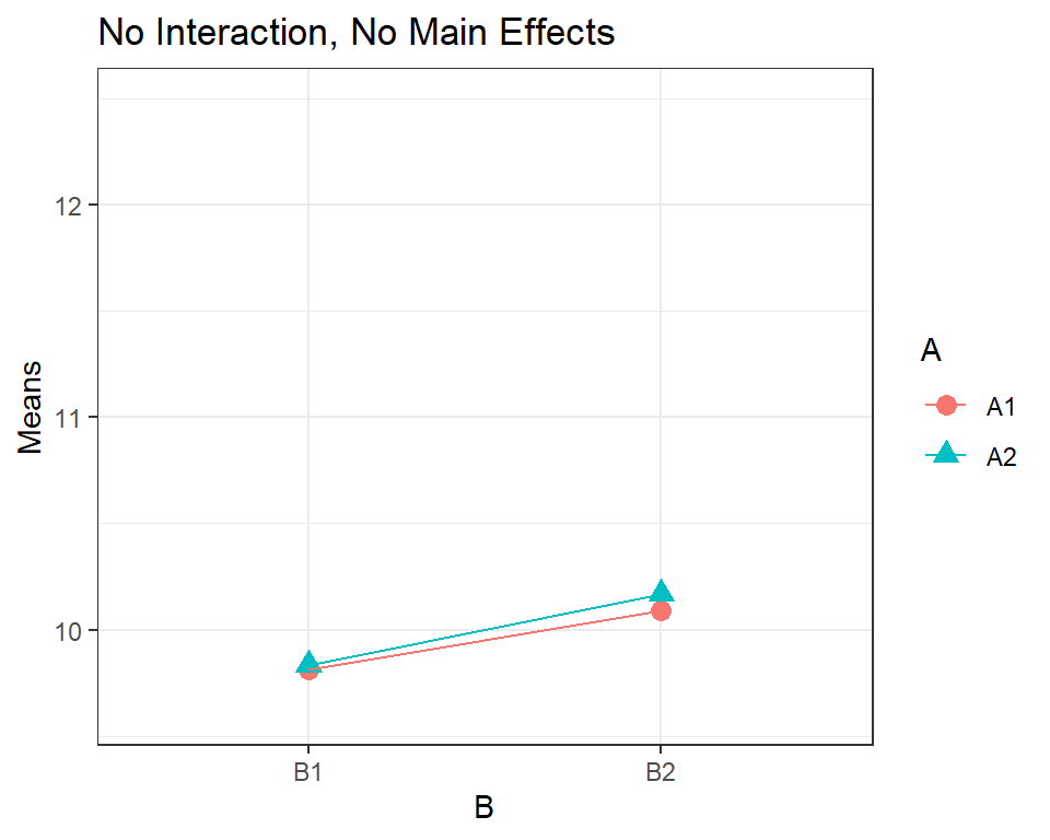

Here there are no significant differences with either Factor $A$ or $B$ .

Now let’s look at a situation with a significant interaction. Remember, if the $F$ test for the interaction term is significant, your explanation and conclusion needs to interpret that interaction and NOT just look at the main effects. Only considering the $F$ tests and the $p$ -values for the factors can be deceiving if a significant interaction is ignored.

## Analysis of Variance Table
## 
## Response: Y
##           Df  Sum Sq Mean Sq F value    Pr(>F)    
## A          1 105.650 105.650 106.982 3.734e-16 ***
## B          1 184.303 184.303 186.625 < 2.2e-16 ***
## A:B        1  69.501  69.501  70.376 1.978e-12 ***
## Residuals 76  75.054   0.988                      
## ---
## Signif. codes:  0 '***' 0.001 '**' 0.01 '*' 0.05 '.' 0.1 ' ' 1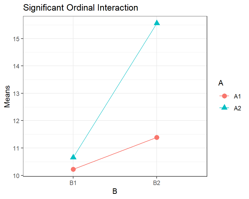

If the farmer uses $B1$ , there is no significant difference in yield between $A1$ and $A2$ , but if the farmer switches to $B2$ , the yield increases significantly more using $A2$ rather than $A1$ .

In some situations, the profiles may even cross, this is called a disordinal interaction. A real-life example might be if planting Seed A rather than Seed B results in a higher yield in one type of soil but a lower yield in the other type of soil.

## Analysis of Variance Table
## 
## Response: Y
##           Df Sum Sq Mean Sq  F value             Pr(>F)    
## A          1   1.81    1.81   1.8636             0.1762    
## B          1  74.05   74.05  76.1390 0.0000000000004475 ***
## A:B        1 501.19  501.19 515.3557          < 2.2e-16 ***
## Residuals 76  73.91    0.97                                
## ---
## Signif. codes:  0 '***' 0.001 '**' 0.01 '*' 0.05 '.' 0.1 ' ' 1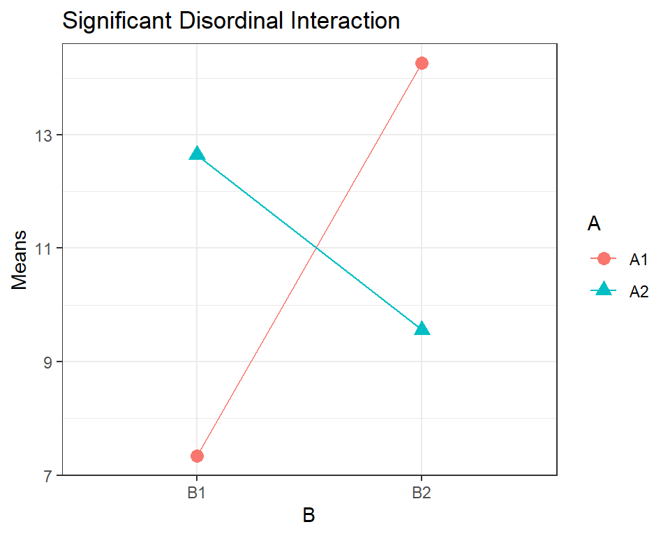

Here, a farmer using $B1$ would have a higher yield using $A2$ , but the pattern reverses and if the farmer switches from $B1$ to $B2$ , they will have a lower yield if they stay with $A2$ .

If Factor $B$ was something like soil type which cannot be easily controlled or changed, then this could drive the farmer’s choice in whether to plant seed $A1$ or $A2$ .