Chapter 11 Categorical Data Analysis
11.1 The Goodness-of-Fit Test
Suppose we have a frequency table and we wish to see if our data fits some hypothetical model. In other words, if \(X\) is our variable, does \(X\) follow a particular distribution? The null hypothesis will state that our observed data does a “good” job of “fitting” some model, and the alternative will be that our data does not “fit” the model.
The technique we will learn for testing for goodness-of-fit (or GOF) is due to Karl Pearson and is called the .
The example we will consider is testing to see if some discrete variable \(X\) “fits” what I call a “generic” probability distribution.
The classic examples which almost all textbooks use are drawn from Mendel’s Theory of Genetics. The monk Gregor Mendel studied traits in pea plants, and his theory stated that if \(A\) represented the seed being smooth (which was the dominant trait) and \(a\) to be that the seed is wrinkled (which is recessive), then he expected the three genotypes AA, Aa, and aa to appear in the ratios \(1:2:1\).
Essentially, the null hypothesis is: \[H_0: \pi_1=1/4, \pi_2=1/2, \pi_3=1/4\]
Rejecting the null hypothesis means that the observed data found by classifying actual peas does NOT fit this hypothetical `generic’ probability distribution.
Let’s consider a dihybrid cross of peas, looking at both color (yellow=dominant,green=recessive) and shape(round=dominant,wrinkled=recessive). A total of \(k=4\) distinct phenotypes are produced.

The four distinct phenotypes produced by our dihybrid cross (as seen in the figure) theoretically occur in the following ratios–9:3:3:1. We obtained a sample of \(n=208\) peas from this dihybrid cross and counted the phenotypes.
| Phenotype | Theoretical Probability | Observed Count |
|---|---|---|
| Yellow, Round | \(\frac{9}{16}\) | 124 |
| Yellow, Wrinkled | \(\frac{3}{16}\) | 30 |
| Green, Round | \(\frac{3}{16}\) | 43 |
| Green, Wrinkled | \(\frac{1}{16}\) | 11 |
This is an extrinsic hypothesis, as Mendelian theory predicts the probabilities before we collect a sample and count the peas.
Step One: Write Hypothesis
\[H_0: p_1=9/16, p_2=3/16, p_3=3/16, p_4=1/16\] \[H_a: \text{At least one equality does not hold}\]
The null hypothesis states that the data fits the Mendelian theory. The alternative hypothesis states that the data deviates significantly from the theory(i.e. the model does NOT fit).
Step Two: Choose Level of Significance
Let \(\alpha=0.05\), the standard choice.
Step Three: Choose Your Test & Check Assumptions
We have chosen the \(\chi^2\) goodness-of-fit test. One assumption that we will need to verify is that all of the expected counts are large enough for the \(\chi^2\) distribution to hold.
The expected counts, or \(E_i\), are the number we would expect to fall in each category \(i\) IF the null hypothesis is true.
For the pea problem, \(E_1=n \times p_1=208 \times 9/16=117\); i.e. we expected 117 round yellow peas.
Similarly, \(E_2=208 \times 3/16=39\), \(E_3=208 \times 3/16=39\), and \(E_4=208 \times 1/16=13\). All of our expected counts are 5 or greater.
If some counts are less than 5, then find the proportion of categories that are less than five. Multiply this proportion by \(k\), which is the number of categories. No expected count should be less than this value.
Step Four: Calculate the Test Statistic
\[\chi^2=\frac{\sum(O_i-E_i)^2}{E_i}\] \[\chi^2=\frac{(124-117)^2}{117}+\frac{(30-39)^2}{39}+\frac{(43-39)^2}{39}+\frac{(11-13)^2}{13}\] \[\chi^2=3.214\] \[df=k-1=4-1=3\]
Step Five: Make a Statistical Decision
We reject the null hypothesis when the \(\chi^2\) test statistic is large. This happens when the observed values do not match the expected values (i.e. the data does not fit the model). If the data was a perfect fit to the model, all \(O_i=E_i\) and \(\chi^2=0\).
From the \(\chi^2\) distribution table, we reject when the test statistic exceeds the critical value \(\chi^2_{k-1,1-\alpha}\) In our case, the critical value is 7.82. Our \(\chi^2\) is smaller, so we fail to reject the null hypothesis at \(\alpha=0.05\)
With technology, you would have with the TI-83/84 or in R. The \(p\)-value is 0.3598.
Step Six: Conclusion
Since we fail to reject the null hypothesis, a proper conclusion would be:
The distribution of phenotypes of the peas does not deviate significantly from Mendelian theory.
11.2 Test of Independence
The \(2 \times 2\) Contingency Table
The contingency table is useful for a cross-tabulation of two categorical variables. In this section, we will concentrate on the \(2 \times 2\) table, with 2 rows and 2 columns when both categorical variables are .
For example, I might classify people on two variables: sex (female or male) and color-blindness (yes or no). We suspect males (XY) are more likely to be color-blind than females (XX) for genetic reasons, i.e. the variables sex and color-blindness are not independent, but are related.
| Sex | Yes | No | Total |
|---|---|---|---|
| Female | 6 | 494 | 500 |
| Male | 44 | 956 | 1000 |
Each of the four entries in the main part of the table are called and \(n_{ij}\) represents an observed count for that cell. For example, \(n_{21}\) is the count in row \(i=2\) and column \(j=1\), which is color-blind males. \(n_{21}=38\).
The two entries in the far right hand column are marginal row totals, denoted as \(n_{i \cdot}\). For example, \(n_{1 \cdot}=500\) is the total for row 1, the number of females.
The first two entries in the bottom row are marginal column totals,denoted as \(n_{\cdot j}\). For example, \(n_{\cdot 2}=956\) is the total for column 2, people that are not color blind.
The final entry in the bottom row is the grand total, denoted as \(n\) or sometimes \(n{\cdot \cdot}\). Here, \(n=1000\).
The \(\chi^2\) Test of Independence
It is often of interest to determine if the two categorical variables in a contingency table are independent. If we reject the null hypothesis of independence, we would conclude that the two variables are associated to a statistically significant degree.
In a \(2 \times 2\) table, this could be determined by using a \(z\)-test for the difference in two proportions. In our problem, we could computed \(p_1\), the proportion of color-blind females, and \(p_2\), the proportion of color-blind males, and determine if the difference in proporitons is significant.
One could also compute a confidence interval for this difference, \(p_1-p_2\).
However, the most common way to test this hypothesis is with a \(\chi^2\) test of independence.
As you will see later, this test can be extended to tables with more than 2 categories per variable.
**Step One: Write Hypotheses
\[H_0: \text{Sex and Color-Blindness are independent}\] \[H_a: \text{Sex and Color-Blindness are NOT independent}\]
Step Two: Choose Level of Significance
Let \(\alpha=0.05\), the standard choice.
Step Three: Choose Test & Check Conditions
We will use the \(\chi^2\) test of independence. We are assuming the data is either a simple random sample of size \(n\) or two independent stratified samples of sizes \(n_{1\cdot}\) and \(n_{2\cdot}\). We need not more than 20% of expected cell counts to be less than 5 and no expected cell counts to be less than one.
Step Four: Compute the Test Statistic
\[\chi^2=\sum_i \sum_j \frac{(O_{ij}-E_{ij})^2}{E_{ij}}\]
\(O_{ij}=n_{ij}\) is the observed count in cell \((i,j)\) and \(E_{ij}=m_{ij}\) is the expected count of that cell, where \[E_{ij}=\frac{n_{i \cdot} \times n_{\cdot j}}{n_{\cdot \cdot}}=\frac{\text{Row Total } \times \text{Column Total}}{\text{Grand Total}}\]
| Sex | Yes | No | Total |
|---|---|---|---|
| Female | 6 | 494 | 500 |
| Male | 44 | 956 | 1000 |
\[E_{11}=\frac{500 \times 44}{1000}=22, E_{12}=\frac{500 \times 956}{1000}=478\] \[E_{21}=\frac{500 \times 44}{1000}=22, E_{22}=\frac{500 \times 956}{1000}=478\]
\[\chi^2=\frac{(6-22)^2}{22}+\frac{(494-478)^2}{478}+\frac{(38-22)^2}{22}+\frac{(462-478)^2}{478}=24.34\] \[df=(r-1)\times(c-1)=1\]
Step Five: Make a Statistical Decision
We have \(\chi^2=24.34\) with \(df=1\) and \(\alpha=0.05\).
From the \(\chi^2\) distribution table, we reject when the test statistic exceeds the critical value \(\chi^2_{1,0.95}\) In our case, the critical value is 3.84. Our \(\chi^2\) is larger, so we reject the null hypothesis at \(\alpha=0.05\)
With technology, you would have with the TI-83/84 or in R. The \(p\)-value is about \(8 \times 10^{-7}\).
Step Six: Conclusion Since we rejected the null hypothesis, a proper conclusion would be:
Sex and color-blindness are significantly associated; they are not independent.
In the observed data, females were much less likely to be color-blind than males, possibly because the genes that produce photopigments that help us see color are found on the X chromosome.
11.3 The Likelihood Ratio \(G\) Test
\(G\)-test The \(G\)-test is a different test statistic that can be used for the test of independence for contingency tables. It is a likelihood ratio test and \(p\)-values are computed using the same degrees of freedom with the chi-square distribution.
\[G=2 \sum_i \sum_j O_{ij} \ln(\frac{O_{ij}}{E_{ij}})\] The idea is that when the null hypothesis is true, \(O_{ij} = E_{ij}\) so the ratio of the two is equal to 1, and the log of 1 is zero, similar to how \((O_{ij}-E_{ij})\) is equal to zero when the null is true.
11.4 Relative Risk (RR) and Odds Ratio (OR)
The rows of the table represent whether a patient has Alzheimer’s or not. The columns represent testing positive or negative for E4, an enzyme that might indicate a genetic risk for Alzheimer’s.
A random sample of 50 individuals at autopsy with Alzheimer’s showed that 18 had E4, while a similar random sample of 200 individuals without Alzheimer’s showed that 24 had E4.
| Positive \(T^+\) | Negative \(T^-\) | ||
|---|---|---|---|
| Alzheimers \(D^+\) | \(a=18\) | \(b=32\) | \(a+b=50\) |
| No Alzheimers \(D^-\) | \(c=24\) | \(d=176\) | \(c+d=200\) |
| \(a+c=42\) | \(b+d=208\) | \(n=a+b+c+d=250\) |
The relative risk gives the rate of disease given exposure/positive test in ratio to the rate of disease given no exposure/negative test.
Or, it could represent the rate of incidence between a treatment vs control (i.e. the physician’s aspirin study).
It is computed as: \[RR=\frac{a(c+d)}{c(a+b)}=\frac{18(200)}{24(50)}=3.0\]
This ratio tells me that Alzheimer’s is 3 times as likely in patients with E4 versus those without E4.
The odds ratio gives the odds of the disease given positive test/exposure in ratio to the odds of the disease given negative test/no exposure. This is similar, but not identical, to the relative risk.
It is computed as \[OR=\frac{a/b}{c/d}=\frac{ad}{bc}=\frac{n_{11} n_{22}}{n_{12} n_{21}}=\frac{18/32}{24/176}=\frac{18(176)}{32(24)}=4.125\]
This ratio indicates that the odds of having Alzheimer’s is over 4 times higher in those with E4 than those without E4.
Rate and odds aren’t equivalent. Relative risk is the ratio of the rate of incidence of disease when exposed/not exposed, while the odds ratio is the ratio of the odds of the incidence of disease when exposed/not exposed.
\(OR\) and \(RR\) seem quite similar, and mathematically \(OR\) converges to \(RR\) when the event is rare. However, \(RR\) is easier to interpret. From Crichton’s Information Point (JCN, 2001):
The odds ratio is used extensively in the healthcare literature. However, few people have a natural ability to interpret odds ratios, except perhaps bookmakers. It is much easier to interpret relative risks. In many situations we will be able to interpret odds ratios by pretending that they are relative risks because, when the events are rare, risks and odds are very similar.
There are statistical reasons to prefer the odds ratio, particularly when fitting certain mathematical models known as logistic regression and Cox regression. These are more sophisticated versions of the linear regression model, appropriate when the response is binary (logistic) or based on survival (Cox)
Confidence intervals for the odds ratio and relative risk are common in the academic literature, particulary in medical studies. The null value of these statistics is 1, so a confidence interval containing 1 indicates a result that is not statistically significant or discernible. Intervals completely below or above 1 indicate a statisticall significant or discernible effect.
The following are findings from an article published in the medical journal The Lancet on March 11, 2020, written by a team of Chinese doctors studying the COVID-19 virus in China.
191 patients (135 from Jinyintan Hospital and 56 from Wuhan Pulmonary Hospital) were included in this study, of whom 137 were discharged and 54 died in hospital. 91 (48%) patients had a comorbidity, with hypertension being the most common (58 [30%] patients), followed by diabetes (36 [19%] patients) and coronary heart disease (15 [8%] patients). Multivariable regression showed increasing odds of in-hospital death associated with older age (odds ratio 1.10, 95% CI 1.03–1.17, per year increase; p=0·0043), …
Notice that the \(OR=1.10\) for age indicates a higher risk of death for older patients, with a confidence interval that lies completely above 1 and a \(p\)-value that is less than \(\alpha=0.05\).
Later in the article are other such results. The sex of the patient was not significant in terms of the odds of death: \(OR=0.61\) (with females having lower odds of death, but not to a statistically significant degree), 95% CI was (0·31–1·20), and the \(p\)-value was 0.15.
The Phi coefficient, \(\Phi\)
An effect size statistic sometimes computed for contingency tables is the phi coefficient. It is computed as the square root of the chi-square test statistic divided by the sample size.
\[\Phi = \sqrt{\frac{\chi^2}{n}}\] The range of \((0,0.3)\) is considered as weak, \((0.3,0.7)\) as medium and \(> 0.7\) as strong.
Effect size statistics such as \(\Phi\) can be useful in judging the practical or clinical significance of a finding, beyond the statistical significance as determining by a \(p\)-value. An example that I computed many years ago dealt with a book that claimed to have “scientific evidence” that astrology can predict many aspects of one’s life. One such claim was that there was a significant association between the astrological signs of members of a married couple. Data from a sample of \(n=358,763\) heterosexual married couples in Switzerland, collected over a seven year period in the 1990s, yielded the following when a chi-square test of independence was used on the \(12 \times 12\) contigency table of the signs of the bride and groom.
\[\chi^2=196.143, df=121, p=0.000018\] A statistically significant result at \(\alpha=0.05\) or \(\alpha=0.01\), admittedly, but the effect size is very small, indicating that the deviations between the observed value and the expected value of marriages of a particular combination of zodiac signs (such as the bride was a Taurus and the groom was a Scorpio) is trivial in size.
\[\Phi = \sqrt{\frac{196.143}{358763}}=0.023\]
Fisher’s Exact Test
This is a permutation test that can be used with contingency tables and is often used when the assumptions for a \(\chi^2\) test in terms of the size of the expected values is violated; that is, when there is an \(E_{ij} < 1\) or more than 20% of those values are less than 5. What happens is that the marginal totals of the contingency table are held constant and the test statistic is computed for all possible tables with those fixed marginal totals. A \(p\)-value is based on comparing the test statistic from the actual data compared to the sampling distribution obtained by considering all such possibilities. This is far too computationally intensive to do by hand. Notice that you will just be provided a \(p\)-value for this. The R function for Fisher’s exact test will also compute the odds ratio and a confidence interval for the odds ratio, based on a more complicated formula than you were shown.
11.5 R Code
In the R code, I use the same example involving Mendel’s peas for the goodness-of-fit test but a couple of different problems for the chi-square test of independence.
# STA 265 Chi-Square Tests
require(tidyverse)
require(mosaic)
require(Stat2Data)
require(MASS)
require(DescTools)

# Goodness of Fit Test
# http://blog.thegrandlocus.com/2016/04/did-mendel-fake-his-results

# https://www.mun.ca/biology/scarr/Dihybrid_Cross.html
# theory: 9/16 Round/Yellow, 3/16 Round/Green,
# 3/16 wrinkled/Yellow, 1/16 wrinkled/green

O.peas <- c(124,30,43,11)
n <- sum(O.peas)
probs <- c(9/16,3/16,3/16,1/16)
E.peas <- n*probs
(X2.stat <- sum((O.peas-E.peas)^2/E.peas))
## [1] 3.213675## [1] 0.3598393##
## Chi-squared test for given probabilities
##
## data: O.peas
## X-squared = 3.2137, df = 3, p-value = 0.3598##
## Chi-squared test for given probabilities
##
## data: x
## X-squared = 3.2137, df = 3, p-value = 0.3598
##
## 124.00 30.00 43.00 11.00
## (117.00) ( 39.00) ( 39.00) ( 13.00)
## [0.42] [2.08] [0.41] [0.31]
## < 0.65> <-1.44> < 0.64> <-0.55>
##
## key:
## observed
## (expected)
## [contribution to X-squared]
## <Pearson residual># the Pearson Residual is sqrt(cell contribution)
# sqrt((O.i-E.i)^2 / E.i), with sign assigned based on O.i-E.i
# Likelihood Ratio Test (aka the G test)
(G.stat <- 2*sum(O.peas*log(O.peas/E.peas)))## [1] 3.390555## [1] 0.3352366##
## Log likelihood ratio (G-test) goodness of fit test
##
## data: O.peas
## G = 3.3906, X-squared df = 3, p-value = 0.3352# repeat with less data
O.peas <- c(24,6,8,2)
# use same theoretical probabilities, Mendelian genetics
xchisq.test(x=O.peas,p=probs)##
## Chi-squared test for given probabilities
##
## data: x
## X-squared = 0.53333, df = 3, p-value = 0.9115
##
## 24.00 6.00 8.00 2.00
## (22.50) ( 7.50) ( 7.50) ( 2.50)
## [0.100] [0.300] [0.033] [0.100]
## < 0.32> <-0.55> < 0.18> <-0.32>
##
## key:
## observed
## (expected)
## [contribution to X-squared]
## <Pearson residual># warning message, 25% or more of cells have E.i < 5
# or any cells with E.i < 1
GTest(x=O.peas,p=probs)##
## Log likelihood ratio (G-test) goodness of fit test
##
## data: O.peas
## G = 0.56017, X-squared df = 3, p-value = 0.9055# what if hypothesis was that each phenotype was equally likely
O.peas <- c(124,30,43,11)
probs <- c(1/4,1/4,1/4,1/4)
xchisq.test(x=O.peas,p=probs)##
## Chi-squared test for given probabilities
##
## data: x
## X-squared = 142.88, df = 3, p-value < 2.2e-16
##
## 124.00 30.00 43.00 11.00
## (52.00) (52.00) (52.00) (52.00)
## [ 99.69] [ 9.31] [ 1.56] [ 32.33]
## < 9.98> <-3.05> <-1.25> <-5.69>
##
## key:
## observed
## (expected)
## [contribution to X-squared]
## <Pearson residual>#############################################################
# Test of Independence
# 2 x 2 table
data(Pima.tr)
Pima <- Pima.tr %>%
mutate(obese=ifelse(bmi>=30,"Obese","Not Obese")) %>%
mutate(type2=recode_factor(type,`Yes`="Type II",`No`="No"))
head(Pima,n=10)## npreg glu bp skin bmi ped age type obese type2
## 1 5 86 68 28 30.2 0.364 24 No Obese No
## 2 7 195 70 33 25.1 0.163 55 Yes Not Obese Type II
## 3 5 77 82 41 35.8 0.156 35 No Obese No
## 4 0 165 76 43 47.9 0.259 26 No Obese No
## 5 0 107 60 25 26.4 0.133 23 No Not Obese No
## 6 5 97 76 27 35.6 0.378 52 Yes Obese Type II
## 7 3 83 58 31 34.3 0.336 25 No Obese No
## 8 1 193 50 16 25.9 0.655 24 No Not Obese No
## 9 3 142 80 15 32.4 0.200 63 No Obese No
## 10 2 128 78 37 43.3 1.224 31 Yes Obese Type II## 'data.frame': 200 obs. of 10 variables:
## $ npreg: int 5 7 5 0 0 5 3 1 3 2 ...
## $ glu : int 86 195 77 165 107 97 83 193 142 128 ...
## $ bp : int 68 70 82 76 60 76 58 50 80 78 ...
## $ skin : int 28 33 41 43 25 27 31 16 15 37 ...
## $ bmi : num 30.2 25.1 35.8 47.9 26.4 35.6 34.3 25.9 32.4 43.3 ...
## $ ped : num 0.364 0.163 0.156 0.259 0.133 ...
## $ age : int 24 55 35 26 23 52 25 24 63 31 ...
## $ type : Factor w/ 2 levels "No","Yes": 1 2 1 1 1 2 1 1 1 2 ...
## $ obese: chr "Obese" "Not Obese" "Obese" "Obese" ...
## $ type2: Factor w/ 2 levels "Type II","No": 2 1 2 2 2 1 2 2 2 1 ...## type2
## obese Type II No
## Not Obese 10 58
## Obese 58 74## [1] 2.987879## rel. risk lwr.ci upr.ci
## 0.3346856 0.1812573 0.5910689## rel. risk lwr.ci upr.ci
## 2.987879 5.517019 1.691850## [1] 4.545946## odds ratio lwr.ci upr.ci
## 0.2199762 0.1034942 0.4675579## odds ratio lwr.ci upr.ci
## 4.545946 9.662376 2.138773##
## Pearson's Chi-squared test with Yates' continuity correction
##
## data: Pima.table
## X-squared = 15.814, df = 1, p-value = 6.988e-05##
## Pearson's Chi-squared test
##
## data: Pima.table
## X-squared = 17.092, df = 1, p-value = 3.561e-05##
## Pearson's Chi-squared test
##
## data: x
## X-squared = 17.092, df = 1, p-value = 3.561e-05
##
## 10 58
## (23.12) (44.88)
## [7.45] [3.84]
## <-2.73> < 1.96>
##
## 58 74
## (44.88) (87.12)
## [3.84] [1.98]
## < 1.96> <-1.41>
##
## key:
## observed
## (expected)
## [contribution to X-squared]
## <Pearson residual>## [1] 0.2923351## [1] 0.2923354# the range of [0, 0.3] is considered as weak,
# [0.3,0.7] as medium and > 0.7 as strong.
fisher.test(Pima.table) # slightly different computation of OR##
## Fisher's Exact Test for Count Data
##
## data: Pima.table
## p-value = 3.314e-05
## alternative hypothesis: true odds ratio is not equal to 1
## 95 percent confidence interval:
## 0.09269285 0.48550819
## sample estimates:
## odds ratio
## 0.2215477tab1 <- Pima.table %>%
as.data.frame() %>%
rownames_to_column() %>%
group_by(obese) %>%
mutate(Prop=Freq/sum(Freq))
tab1## # A tibble: 4 × 5
## # Groups: obese [2]
## rowname obese type2 Freq Prop
## <chr> <fct> <fct> <int> <dbl>
## 1 1 Not Obese Type II 10 0.147
## 2 2 Obese Type II 58 0.439
## 3 3 Not Obese No 58 0.853
## 4 4 Obese No 74 0.561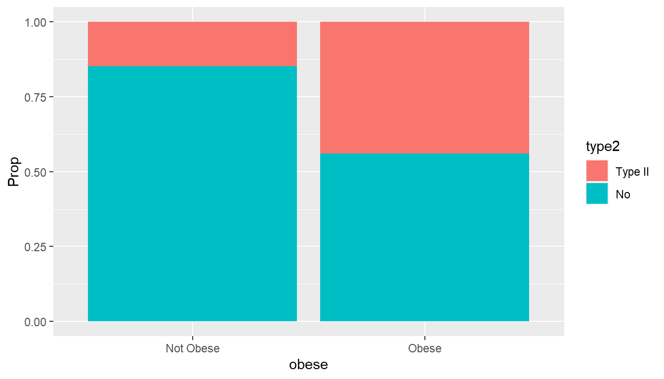
#######################################################
# table beyond 2x2 table
# ice cream preference
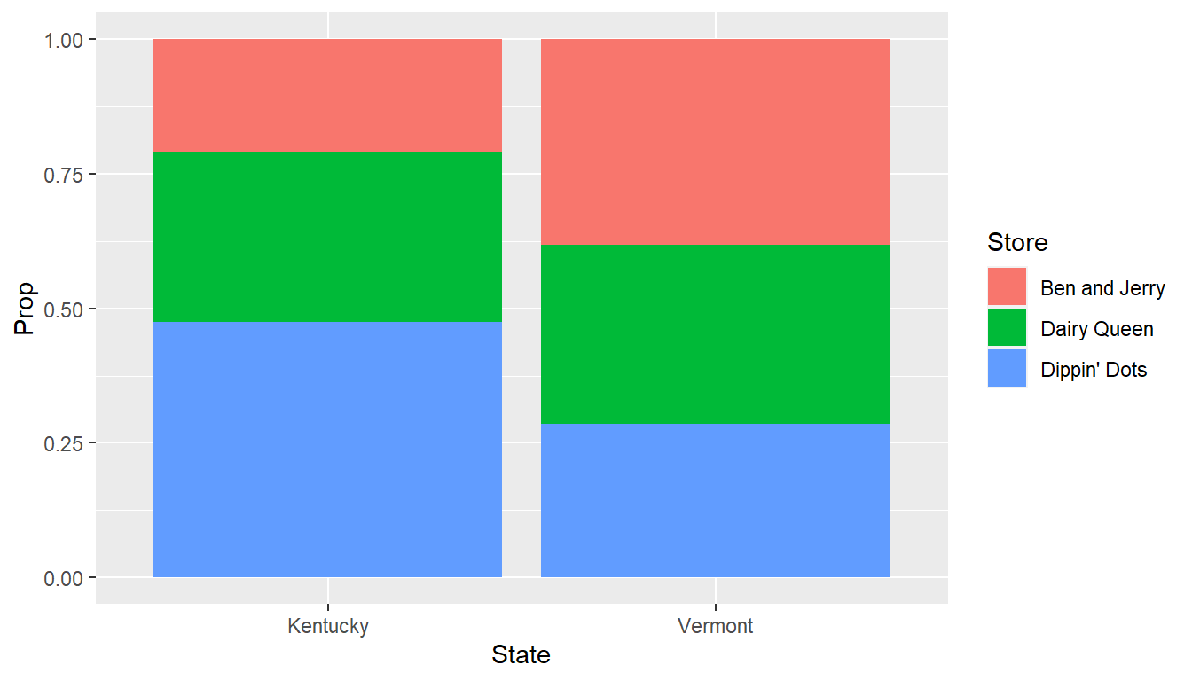
icecream.table <- rbind(Kentucky=c(25,38,57),
Vermont=c(48,42,36))
colnames(icecream.table) <- c("Ben and Jerry","Dairy Queen",
"Dippin' Dots")
icecream.table## Ben and Jerry Dairy Queen Dippin' Dots
## Kentucky 25 38 57
## Vermont 48 42 36##
## Pearson's Chi-squared test
##
## data: x
## X-squared = 12.049, df = 2, p-value = 0.002418
##
## 25.00 38.00 57.00
## (35.61) (39.02) (45.37)
## [3.161] [0.027] [2.984]
## <-1.78> <-0.16> < 1.73>
##
## 48.00 42.00 36.00
## (37.39) (40.98) (47.63)
## [3.011] [0.026] [2.842]
## < 1.74> < 0.16> <-1.69>
##
## key:
## observed
## (expected)
## [contribution to X-squared]
## <Pearson residual>## [1] 0.2213166# Cramer's V = sqrt((chisq/n)/min(r-1,c-1))
# extension of Phi for beyond 2x2 table
# https://www.ncbi.nlm.nih.gov/pmc/articles/PMC5426219/
# look at Table 2
fisher.test(icecream.table)##
## Fisher's Exact Test for Count Data
##
## data: icecream.table
## p-value = 0.002419
## alternative hypothesis: two.sided# visualize
tab2 <- icecream.table %>%
as.data.frame() %>%
rownames_to_column() %>%
gather(Column,Value,-rowname) %>%
transmute(State=rowname,Store=Column,Freq=Value) %>%
group_by(State) %>%
mutate(Prop=Freq/sum(Freq))
tab2## # A tibble: 6 × 4
## # Groups: State [2]
## State Store Freq Prop
## <chr> <chr> <dbl> <dbl>
## 1 Kentucky Ben and Jerry 25 0.208
## 2 Vermont Ben and Jerry 48 0.381
## 3 Kentucky Dairy Queen 38 0.317
## 4 Vermont Dairy Queen 42 0.333
## 5 Kentucky Dippin' Dots 57 0.475
## 6 Vermont Dippin' Dots 36 0.286