Chapter 2 Inference for Simple Linear Regression

2.1 The ANOVA Table for Simple Regression

In this chapter, we consider statistical inference, including both confidence intervals and hypothesis testing, in simple linear regression.

While it is possible to conduct inference on both the intercept parameter $\beta_0$ and the slope parameter $\beta_1$, we will focus on the slope since our interest is usually in the strength of the linear relationship (i.e. correlation) between two variables. We will also look at some types of intervals that look at the margin of error for predicted values.

Some useful formulas: $$\hat{Y} = \hat{\beta}_0 + \hat{\beta}_1 X$$

$$SSTotal = \sum(Y-\bar{Y})^2, SSModel = \sum(\hat{Y}-\bar{Y})^2, SSE = SSError = \sum(Y-\hat{Y})^2$$

$$SSTotal = SSModel + SSError$$ Note: These appear with many different names. In particular, R will label $SSE$ as Residuals.

ANOVA Table for simple linear regression:

Source	$df$	$SS$	$MS$	$F$	$p$-value
Model	1	$SSModel$	$MSModel$	$F$	$p$-value
Errror	$n-2$	$SSE$	$MSE$
Total	$n-1$	$SSTotal$

For simple linear regression (these will change when we go into multiple linear regression and use more than 1 predictor $X$ variable)

$$MSModel = \frac{SSModel}{1}, MSE = \frac{SSE}{n-2}$$ Note that $MSE=\hat{\sigma}^2_\epsilon$ and thus the root MSE is $\sqrt{MSE}=\hat{\sigma}_\epsilon$ Many books will use $S_{Y|X}$ to represent this quantity instead, and R calls it Residual standard error and your book calls it standard error of regression.

The overall $F$ statistic for the model is: $$F=\frac{MSModel}{MSE}, df=1,n-2$$ which will be equal to 1 if the null hypothesis is true where both $MSModel$ and $MSE$ are independent estimates of total response variance $\sigma^2$. Note unlike the standard normal or $t$ distributions that the $F$ distribution only takes on positive values and the $p$-value is one-sided.

2.2 Inference For The Slope

$$SSX = \sum(x-\bar{x})^2 = (n-1)s_x^2, SSXY = \sum(x-\bar{x})(y-\bar{y})$$ $$\hat{\beta}_1 = \frac{SSXY}{SSX}, \hat{\beta}_0 = \bar{y} - \hat{\beta}_1 \bar{x}$$ Standard Errors: $$s_{\hat{\beta}_1}=SE_{\hat{\beta}_1}=\frac{\sqrt{MSE}}{\sqrt{SSX}}$$

If we are testing for the statisical significance of the slope of a simple linear regression equation, then $$H_O: \beta_1=0, H_a: \beta_1 \neq 0$$ $$t=\frac{\hat{\beta}_1}{SE_{\hat{\beta}_1}}, df=n-2$$

For simple linear regression, an equivalent test for the correlation between the predictor $X$ and the response $Y$ is:

$$H_O: \rho = 0 , H_a: \rho \neq 0$$ $$t=\frac{r\sqrt{n-2}}{\sqrt{1-r^2}}, df=n-2$$ Note: $t^2 = F$ when $t \sim t(\eta)$ and $F \sim F(1,\eta)$. In other words, for simple linear regression, we can square the $t$ statistic, obtain the $F$ statistic from the ANOVA table, and the $p$-values will be identical.

Coefficient of determination, or the Multiple R-squared statistic:

$$R^2 = \frac{SSModel}{SSTotal}=1-\frac{SSError}{SSTotal}$$ Confidence Intervals:

The slope $\beta_1$:

$$\hat{\beta}_1 \pm t^* {SE_{\hat{\beta}_1}}$$

where $t^*$ is the critical value from the $t$ distribution for $n-2$ df and the $100(1-\alpha)$ percent confidence interval. Usually we use 95% CI, so $\alpha=0.05$.

2.3 Confidence and Prediction Bands

The “confidence band”, which is a confidence interval for the mean response $\mu_{Y|X^*}$:

$$\hat{y} \pm t^* SE_{\hat{\mu}}$$

$$SE_{\hat{\mu}}=\hat{\sigma}_\epsilon \sqrt{\frac{1}{n}+\frac{(x^*-\bar{x})^2}{\sum(x-\bar{x})^2}}$$ The “prediction band”, which is a confidence interval for an individual predicted vale $\hat{y}_{X^*}$ is:

$$\hat{y} \pm t^* SE_{\hat{y}}$$

$$SE_{\hat{y}}=\hat{\sigma}_\epsilon \sqrt{1+\frac{1}{n}+\frac{(x^*-\bar{x})^2}{\sum(x-\bar{x})^2}}$$

2.4 R Code, Galton’s Height Data

# Chapter 2 Code

require(tidyverse)
require(mosaic) # for favstats() and Galton data set
data(Galton)
# look at relationship between the height of a man and his father
# "regression towards the mean"

boys <- Galton %>%
  filter(sex=="M") %>%
  mutate(hgt=2.54*height,dad=2.54*father,mom=2.54*mother)

model2 <- lm(height~father,data=boys) # in inches
model2

## 
## Call:
## lm(formula = height ~ father, data = boys)
## 
## Coefficients:
## (Intercept)       father  
##     38.2589       0.4477

model3 <- lm(hgt~dad,data=boys) # in cm
model3

## 
## Call:
## lm(formula = hgt ~ dad, data = boys)
## 
## Coefficients:
## (Intercept)          dad  
##     97.1776       0.4477

# scatterplot, basic descriptive statistics
# done in inches
favstats(~height,data=boys)

##  min   Q1 median Q3 max     mean       sd   n missing
##   60 67.5   69.2 71  79 69.22882 2.631594 465       0

favstats(~father,data=boys)

##  min Q1 median   Q3  max     mean       sd   n missing
##   62 68     69 70.5 78.5 69.16817 2.299929 465       0

ggplot(boys,aes(x=father,y=height)) + geom_point()

## Analysis of Variance Table by hand
yhat <- fitted(model2)
Y <- boys$height
X <- boys$father
ybar <- mean(Y)
xbar <- mean(X)

SSTotal <- sum((Y-ybar)^2)
SSModel <- sum((yhat-ybar)^2)
SSE <- sum((Y-yhat)^2)
SSTotal

## [1] 3213.334

SSModel

## [1] 492.0555

n <- nrow(boys)
MSModel <- SSModel/1
MSModel

## [1] 492.0555

MSE <- SSE/(n-2)
MSE

## [1] 5.877491

SSX <- sum((X-xbar)^2)
SSXY <- sum((X-xbar)*(Y-ybar))
beta.hat1 <- SSXY/SSX
beta.hat1

## [1] 0.4477479

SE.beta.hat1 <- sqrt(MSE)/sqrt(SSX)
SE.beta.hat1

## [1] 0.04893533

# confidence interval for the slope
alpha <- 0.05 # 95% confidence
t.star <- qt(p=1-alpha/2,df=n-2)
beta.hat1 + c(-1,1)*t.star*SE.beta.hat1

## [1] 0.3515851 0.5439108

# t statistics for slope, df=n-2
t.stat <- beta.hat1/SE.beta.hat1
t.stat

## [1] 9.149788

p.valT<-2*pt(abs(t.stat),df=n-2,lower.tail=FALSE)
p.valT

## [1] 1.824016e-18

# t statistic for the correlation between Y and X, df=n-2
r <- cor(height~father,data=boys)
t.stat2<-(r*sqrt(n-2))/sqrt(1-r^2)
t.stat2

## [1] 9.149788

# F statistic for the regression model, df=1,n-2           
F.stat<-MSModel/MSE
F.stat

## [1] 83.71863

p.valF<-pf(F.stat,df1=1,df2=n-2,lower.tail=FALSE)
p.valF

## [1] 1.824016e-18

# base functions for summarizing a regression model
coefficients(model2)

## (Intercept)      father 
##  38.2589122   0.4477479

summary(model2)

## 
## Call:
## lm(formula = height ~ father, data = boys)
## 
## Residuals:
##     Min      1Q  Median      3Q     Max 
## -9.3774 -1.4968  0.0181  1.6375  9.3987 
## 
## Coefficients:
##             Estimate Std. Error t value Pr(>|t|)    
## (Intercept) 38.25891    3.38663   11.30   <2e-16 ***
## father       0.44775    0.04894    9.15   <2e-16 ***
## ---
## Signif. codes:  0 '***' 0.001 '**' 0.01 '*' 0.05 '.' 0.1 ' ' 1
## 
## Residual standard error: 2.424 on 463 degrees of freedom
## Multiple R-squared:  0.1531, Adjusted R-squared:  0.1513 
## F-statistic: 83.72 on 1 and 463 DF,  p-value: < 2.2e-16

summary(model3) # what's the same and what's different with cm rather than inches

## 
## Call:
## lm(formula = hgt ~ dad, data = boys)
## 
## Residuals:
##     Min      1Q  Median      3Q     Max 
## -23.819  -3.802   0.046   4.159  23.873 
## 
## Coefficients:
##             Estimate Std. Error t value Pr(>|t|)    
## (Intercept) 97.17764    8.60205   11.30   <2e-16 ***
## dad          0.44775    0.04894    9.15   <2e-16 ***
## ---
## Signif. codes:  0 '***' 0.001 '**' 0.01 '*' 0.05 '.' 0.1 ' ' 1
## 
## Residual standard error: 6.158 on 463 degrees of freedom
## Multiple R-squared:  0.1531, Adjusted R-squared:  0.1513 
## F-statistic: 83.72 on 1 and 463 DF,  p-value: < 2.2e-16

anova(model2)

## Analysis of Variance Table
## 
## Response: height
##            Df  Sum Sq Mean Sq F value    Pr(>F)    
## father      1  492.06  492.06  83.719 < 2.2e-16 ***
## Residuals 463 2721.28    5.88                      
## ---
## Signif. codes:  0 '***' 0.001 '**' 0.01 '*' 0.05 '.' 0.1 ' ' 1

confint(model2)

##                  2.5 %     97.5 %
## (Intercept) 31.6038348 44.9139896
## father       0.3515851  0.5439108

# newer functions for summarizing a regression model
require(broom)
tidy(model2)

## # A tibble: 2 × 5
##   term        estimate std.error statistic  p.value
##   <chr>          <dbl>     <dbl>     <dbl>    <dbl>
## 1 (Intercept)   38.3      3.39       11.3  2.64e-26
## 2 father         0.448    0.0489      9.15 1.82e-18

glance(model2)

## # A tibble: 1 × 12
##   r.squared adj.r.squared sigma statistic  p.value    df logLik   AIC   BIC
##       <dbl>         <dbl> <dbl>     <dbl>    <dbl> <dbl>  <dbl> <dbl> <dbl>
## 1     0.153         0.151  2.42      83.7 1.82e-18     1 -1071. 2147. 2160.
## # ℹ 3 more variables: deviance <dbl>, df.residual <int>, nobs <int>

augment(model2) %>%
  ggplot(aes(.fitted,.resid)) + geom_point() +
  geom_hline(yintercept=0,col="red",linetype="dashed")# residual plot

#confidence band, prediction band
# 95% confidence band (i.e. interval for the mean response) is in gray
# if X = 66, this is a CI for the average height of all men
# with a father that is 66 inches tall (I am one such person)

ggplot(boys, aes(x=father,y=height)) +
  geom_point() +
  geom_smooth(method=lm, se=TRUE) +  #try method=loess
  geom_vline(xintercept=66,color="blue",linetype="dotted")

# create the 90% prediction band, store values, plot
# if X = 66, this is a PI for the average height of a particular
# man with a father that is 66 inches tall (such as me)
N <- nrow(boys)
new <- data.frame(father=seq(60,80,length.out=N))
PI <- predict(model2, new, interval="prediction",level=0.90)  
# can do interval="confidence" instead, default level is 0.95

new_dat <- cbind(new, PI)
# combine these two data sets together
head(new_dat)

##     father      fit      lwr      upr
## 1 60.00000 65.12379 61.05602 69.19156
## 2 60.04310 65.14309 61.07595 69.21022
## 3 60.08621 65.16239 61.09588 69.22890
## 4 60.12931 65.18169 61.11580 69.24757
## 5 60.17241 65.20099 61.13572 69.26625
## 6 60.21552 65.22028 61.15564 69.28493

ggplot(boys,aes(x=father,y=height)) +
  geom_point() +
  geom_smooth(method=lm,se=TRUE,level=0.90) +
  geom_line(data=new_dat,aes(x=father,y=lwr), color = "red", linetype = "dashed")+
  geom_line(data=new_dat,aes(x=father,y=upr), color = "red", linetype = "dashed")+
  geom_vline(xintercept=66,color="blue",linetype="dotted")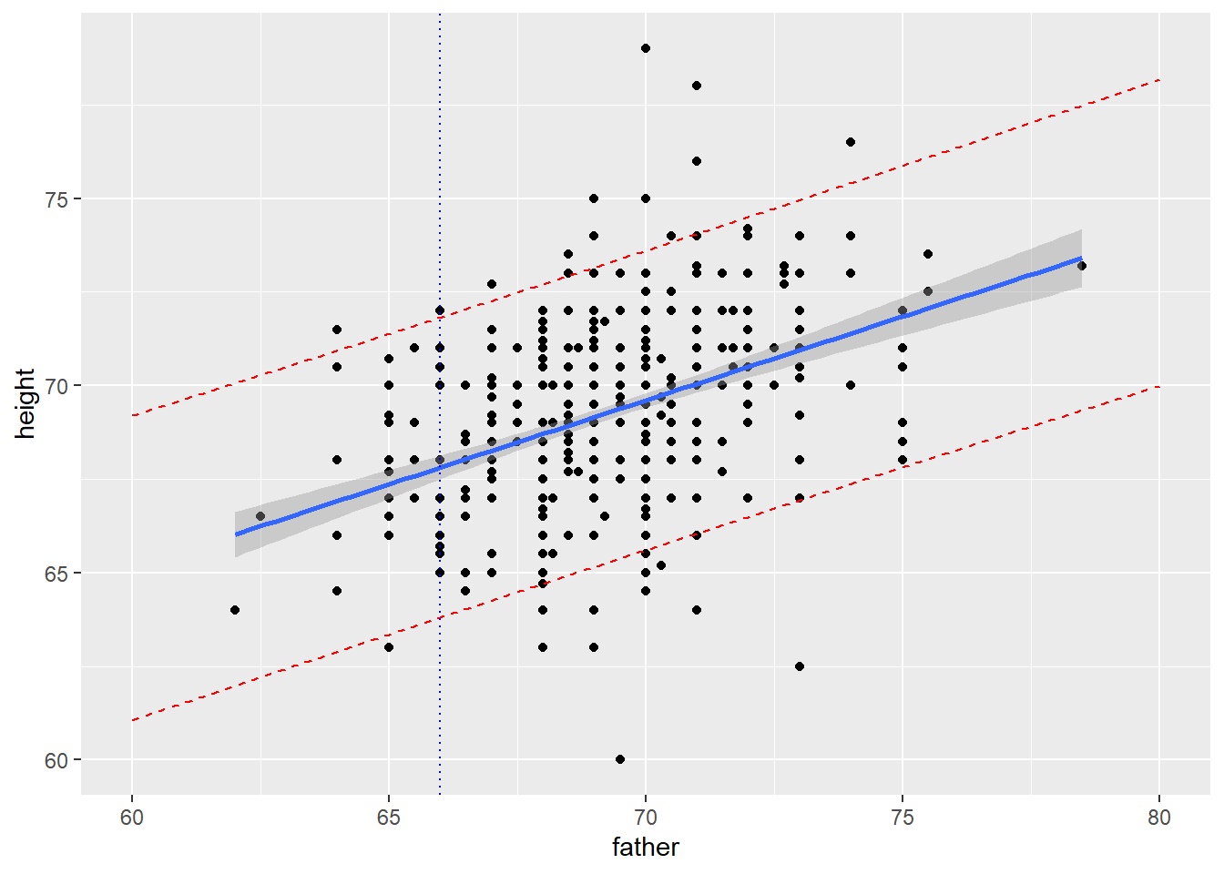

2.5 Confidence and Prediction Bands, Books Example

Let’s fit a simple linear regression model to predict the price of a textbook, based on the number of pages. (This is problem 2.16 from the textbook)

Suppose we need to compute the “confidence band” (the 95% CI for the mean response) and/or “prediction band” (the 95% CI for a predicted value) for a specific value of $X$, say $X^* = 450$ pages. (This is problem 2.44 from the textbook)

$$\hat{Y}=-3.42231 + 0.14733(450)=\$62.88$$

Confidence band: $$\hat{Y} \pm t^* \sqrt{MSE} \sqrt{\frac{1}{n}+\frac{(X^*-\bar{X})}{(n-1)s^2_x}}$$

Prediction band: $$\hat{Y} \pm t^* \sqrt{MSE} \sqrt{1+\frac{1}{n}+\frac{(X^*-\bar{X})}{(n-1)s^2_x}}$$

$$t^*=2.048407, df=n-2=28$$

$$MSE=886, \sqrt{MSE}=\hat{\sigma_\epsilon}=RMSE=29.76$$

$$n=30, \bar{X}=464.5333, s_x^2=82414.53$$

require(tidyverse)
require(Stat2Data)
require(broom)

# Problem 2.44
# fit model, draw the confidence and prediction bands

data(TextPrices)
text.model <- lm(Price~Pages,data=TextPrices)
summary(text.model)

## 
## Call:
## lm(formula = Price ~ Pages, data = TextPrices)
## 
## Residuals:
##     Min      1Q  Median      3Q     Max 
## -65.475 -12.324  -0.584  15.304  72.991 
## 
## Coefficients:
##             Estimate Std. Error t value Pr(>|t|)    
## (Intercept) -3.42231   10.46374  -0.327    0.746    
## Pages        0.14733    0.01925   7.653 2.45e-08 ***
## ---
## Signif. codes:  0 '***' 0.001 '**' 0.01 '*' 0.05 '.' 0.1 ' ' 1
## 
## Residual standard error: 29.76 on 28 degrees of freedom
## Multiple R-squared:  0.6766, Adjusted R-squared:  0.665 
## F-statistic: 58.57 on 1 and 28 DF,  p-value: 2.452e-08

anova(text.model)

## Analysis of Variance Table
## 
## Response: Price
##           Df Sum Sq Mean Sq F value    Pr(>F)    
## Pages      1  51877   51877  58.573 2.452e-08 ***
## Residuals 28  24799     886                      
## ---
## Signif. codes:  0 '***' 0.001 '**' 0.01 '*' 0.05 '.' 0.1 ' ' 1

N <- nrow(TextPrices)
new <- data.frame(Pages=seq(0,1100,length.out=N))
PI <- predict(text.model, new, interval="prediction") # 95% PI
new_dat <- cbind(new,PI)

ggplot(TextPrices,aes(x=Pages,y=Price)) + geom_point(col="blue") +
  geom_smooth(method=lm,se=TRUE) + # line and confidence band
  geom_line(data=new_dat,aes(x=Pages,y=lwr),color="red",linetype="dashed") + 
  geom_line(data=new_dat,aes(x=Pages,y=upr),color="red",linetype="dashed") +
  geom_vline(xintercept=450,col="green4",linetype="dashed") +
  annotate("text",label="X* = 450 pages",x=400,y=-50,color="green4")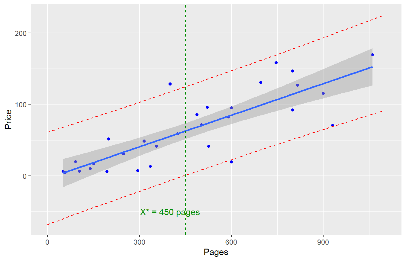

# CI for mean response when X*=450 (i.e. the confidence band)
yhat <- -3.42231+0.14733*450 # yhat is $62.88
n <- nrow(TextPrices)
tstar <- qt(p=0.975,df=n-2) #t*=2.048407, critical value
RMSE <- sqrt(886) # residual standard error, sqrt(MSE) or sigma-hat_epsilon
xstar <- 450
xbar <- mean(TextPrices$Pages) 
varx <- var(TextPrices$Pages) 

# confidence band for mean response when X*=450

yhat + c(-1,1)*tstar*RMSE*sqrt(1/n + ((xstar-xbar)^2/(varx*(n-1))))

## [1] 51.72946 74.02292

# PI for individual prediction when X*=450 (i.e. the prediction band)

yhat + c(-1,1)*tstar*RMSE*sqrt(1 + 1/n + ((xstar-xbar)^2/(varx*(n-1))))

## [1]   0.8932842 124.8590958

# PI for individual prediction when X*=1500 (i.e. the prediction band)

xstar <- 1500
yhat + c(-1,1)*tstar*RMSE*sqrt(1 + 1/n + ((xstar-xbar)^2/(varx*(n-1))))

## [1] -11.34863 137.10101

# not too confident in this since this is extrapolating beyond the range of data
# the linear trend/rate of change might not hold for very large books
# like Chelsea's Norton Anthology of Literature (I had one of those back in the day)

# also, as e-books get more popular as college textbooks, that could change
# the relationship