Chapter 3 Multiple Linear Regression
3.1 The Model
We can extend the simple linear regression model to the situation where we have \(k\) predictor variables \(X_1,X_2,\cdots,X_k\) and a response variable \(Y\). Think of simple linear regression as the special case where \(k=1\), the graph of the data is a 2-D scatterplot, and the least squares regression model is merely the equation of a straight line.
\[Y_i = \beta_0 + \beta_1 X_{1i} + \beta_2 X_{2i} + \cdots + \beta_k X_{ki} + \epsilon_i\] or \[Y_i = \beta_0 + \sum_{j=1}^k \beta_i X_{ji} + \epsilon_i\] We still make the same assumptions as before. Note that the variable \(Y\) is normally distributed with variance \(\sigma^2\) for each combination of \(X_1,X_2,\cdots,X_K\), or equivalently \(\epsilon \sim N(0,\sigma^2)\). If \(k=2\) (i.e. exactly 2 predictors), the scatterplot will be in 3-D and we will fit the least squares regression plane to the data. When \(k \geq 3\), we fit a regression surface (often called a response surface). If we let some \(X_j\) be higher-odrder functions of the basic independent variables (i.e. something like \(X_3 =X_2^2\) or \(X_4 = X_1 X_2\)), the response surface will be nonlinear.
3.2 The AccordPrices Example
Let’s put this is action using the AccordPrice data set in the Stat2Data package, where we will predict Price using both the car’s Age and its Mileage. I’ll install the GGally package to help with some plotting.
require(tidyverse)
require(GGally)
require(Stat2Data)
data(AccordPrice)
ggpairs(AccordPrice) # from GGally
##
## Call:
## lm(formula = Price ~ Age + Mileage, data = AccordPrice)
##
## Residuals:
##     Min      1Q  Median      3Q     Max
## -4.5832 -1.5016 -0.1708  0.9218  6.8996
##
## Coefficients:
##             Estimate Std. Error t value Pr(>|t|)
## (Intercept) 21.73825    0.72194   30.11  < 2e-16 ***
## Age         -0.79138    0.15764   -5.02 2.88e-05 ***
## Mileage     -0.05315    0.01682   -3.16  0.00387 **
## ---
## Signif. codes:  0 '***' 0.001 '**' 0.01 '*' 0.05 '.' 0.1 ' ' 1
##
## Residual standard error: 2.259 on 27 degrees of freedom
## Multiple R-squared:  0.8555, Adjusted R-squared:  0.8448
## F-statistic: 79.96 on 2 and 27 DF,  p-value: 4.532e-12
I doubt you are surprised that both Age and Mileage are negatively correlated with the Price, while they are positively corrleated with each other. The \(t\)-tests for both Age and Mileage are statistically signficiant at a traditional level of \(\alpha=0.05\)
Age: \(t=-5.02\), \(df=27\), \(p<.0001\)
Mileage: \(t=-3.16\), \(df=27\), \(p=.0039\)
A relatively simple measure of the “quality” of a regression model is \(R^2\). This was just the squared correlation in simple linear regression. Now, it is the squared multiple correlation coefficient between the variables \(Y, X_1, \cdots, X_K\). It can be computed from the sum of squares as:
\[R^2 = \frac{SSModel}{SSY} = 1 - \frac{SSE}{SSY}\]
Note that the multiple \(R^2\) for our two-variable regression model for predicting the price of a Honda Accord is \(R^2=0.8555\). Over 85% of the variation in the price of the used car is acccounted for by this linear model that uses the car’s age and mileage.
The two simple linear regression models return \(r^2=0.8021\) (for Age) and \(r^2=0.7207\) (for Mileage). A flaw of the multiple \(R^2\) statistic is that it will always increase when a new predictor \(X_j\) is added to the model, even if it has virtually no correlation with \(Y\), such as the last digit of the car’s VIN number.
A variation called Adjusted \(R^2\) is also computed by R with the formula
\[\text{Adjusted } R^2 = 1 - \frac{(1-R^2)(n-1)}{n-k-1}\]
This formula is a crude way to “penalize” a model for becoming more complicated with the addition of \(\beta_j\) terms (slopes for new variables). The Principle of Parsimony tells us that we want the simplest model that adequately explains a phenonmenon. We’ll see better ways of selecting a model in future weeks.
3.3 The airquality Example
Let’s look at the airquality example from base R. There are \(k=3\) predictors where the direction of the relationship between the response Ozone (the ozone level, measured in parts per billion) and the predictors Solar.R (in langleys), Wind (average wind speed in miles per hour), and Temp (maximum daily temperature in degrees Fahrenheit). I’ll ignore the Month and Day variables in my regression model. Notice that many data values are missing and denoted as NA in the data set.
From the scatterplot matrix, we see that the Ozone level is positively correleated with Solar.R and Temp but is negatively correlated with Wind. I’m going to fit the multiple regression model, provide the summary which will have \(t\)-tests on each \(X_j\), and the ANOVA tables computed with both the anova and Anova functions (which will be different, unlike simple linear regression!)
I’m going to create a data set with all of the observations with missing data values NA removed. Also, we will learn about Type I and Type II Sums of squares and when you would choose one or the other.
# create a data set with all cases with missing data removed
aq.data <- airquality %>%
  drop_na()

summary(aq.data)
## Ozone Solar.R Wind Temp
## Min. : 1.0 Min. : 7.0 Min. : 2.30 Min. :57.00
## 1st Qu.: 18.0 1st Qu.:113.5 1st Qu.: 7.40 1st Qu.:71.00
## Median : 31.0 Median :207.0 Median : 9.70 Median :79.00
## Mean : 42.1 Mean :184.8 Mean : 9.94 Mean :77.79
## 3rd Qu.: 62.0 3rd Qu.:255.5 3rd Qu.:11.50 3rd Qu.:84.50
## Max. :168.0 Max. :334.0 Max. :20.70 Max. :97.00
## Month Day
## Min. :5.000 Min. : 1.00
## 1st Qu.:6.000 1st Qu.: 9.00
## Median :7.000 Median :16.00
## Mean :7.216 Mean :15.95
## 3rd Qu.:9.000 3rd Qu.:22.50
## Max. :9.000 Max. :31.00## min Q1 median Q3 max mean sd n missing
## 1 18 31.5 63.25 168 42.12931 32.98788 116 37## min Q1 median Q3 max mean sd n missing
## 1 18 31 62 168 42.0991 33.27597 111 0##
## Call:
## lm(formula = Ozone ~ Solar.R + Temp + Wind, data = aq.data)
##
## Residuals:
## Min 1Q Median 3Q Max
## -40.485 -14.219 -3.551 10.097 95.619
##
## Coefficients:
## Estimate Std. Error t value Pr(>|t|)
## (Intercept) -64.34208 23.05472 -2.791 0.00623 **
## Solar.R 0.05982 0.02319 2.580 0.01124 *
## Temp 1.65209 0.25353 6.516 2.42e-09 ***
## Wind -3.33359 0.65441 -5.094 1.52e-06 ***
## ---
## Signif. codes: 0 '***' 0.001 '**' 0.01 '*' 0.05 '.' 0.1 ' ' 1
##
## Residual standard error: 21.18 on 107 degrees of freedom
## Multiple R-squared: 0.6059, Adjusted R-squared: 0.5948
## F-statistic: 54.83 on 3 and 107 DF, p-value: < 2.2e-16## Analysis of Variance Table
##
## Response: Ozone
## Df Sum Sq Mean Sq F value Pr(>F)
## Solar.R 1 14780 14780 32.944 8.946e-08 ***
## Temp 1 47378 47378 105.607 < 2.2e-16 ***
## Wind 1 11642 11642 25.950 1.516e-06 ***
## Residuals 107 48003 449
## ---
## Signif. codes: 0 '***' 0.001 '**' 0.01 '*' 0.05 '.' 0.1 ' ' 1## Anova Table (Type II tests)
##
## Response: Ozone
## Sum Sq Df F value Pr(>F)
## Solar.R 2986 1 6.6563 0.01124 *
## Temp 19050 1 42.4630 2.424e-09 ***
## Wind 11642 1 25.9495 1.516e-06 ***
## Residuals 48003 107
## ---
## Signif. codes: 0 '***' 0.001 '**' 0.01 '*' 0.05 '.' 0.1 ' ' 1Recall we compute sums of squares with:
\[SSY = \sum_{i=1}^n (Y-\bar{Y})^2\]
\[SSModel = \sum_{i=1}^n (\hat{Y}-\bar{Y})^2\] \[SSE = \sum_{i=1}^n (Y-\hat{Y})^2\]
The anova function with the lower case a computes what are known as Type I SS, also called “variables-added-in-order” or sequential sums of squares. These are used when the sequence of adding the \(X\) variables into the model is important to us.
Both the summary and Anova functions (upper case A) computes what are known as Type II SS, also called “variables-added-last” or unique sums of squares. These are used when the sequence of adding the \(X\) variables into the model is arbitrary, and our interest instead is on whether that particular \(X\) variable makes a contribution to explaining the variability of \(Y\) above and beyond all of the other \(X\) variables. The summary table presents them as partial \(t\)-statistics, while the Anova table presents them as partial \(F\)-statistics. Notice the \(p\)-values are identical and \(t^2=F\) for a particular \(X\) variable, where the \(t\)-test has \(df=n-k-1\) and the \(F\)-test has \(df=1,n-k-1\).
# let's see what happens if I enter the 3 X variables in a different order
aq.mixed <- lm(Ozone ~ Wind + Solar.R + Temp,data=aq.data)
summary(aq.mixed) # unchanged
##
## Call:
## lm(formula = Ozone ~ Wind + Solar.R + Temp, data = aq.data)
##
## Residuals:
## Min 1Q Median 3Q Max
## -40.485 -14.219 -3.551 10.097 95.619
##
## Coefficients:
## Estimate Std. Error t value Pr(>|t|)
## (Intercept) -64.34208 23.05472 -2.791 0.00623 **
## Wind -3.33359 0.65441 -5.094 1.52e-06 ***
## Solar.R 0.05982 0.02319 2.580 0.01124 *
## Temp 1.65209 0.25353 6.516 2.42e-09 ***
## ---
## Signif. codes: 0 '***' 0.001 '**' 0.01 '*' 0.05 '.' 0.1 ' ' 1
##
## Residual standard error: 21.18 on 107 degrees of freedom
## Multiple R-squared: 0.6059, Adjusted R-squared: 0.5948
## F-statistic: 54.83 on 3 and 107 DF, p-value: < 2.2e-16## Analysis of Variance Table
##
## Response: Ozone
## Df Sum Sq Mean Sq F value Pr(>F)
## Wind 1 45694 45694 101.854 < 2.2e-16 ***
## Solar.R 1 9055 9055 20.184 1.786e-05 ***
## Temp 1 19050 19050 42.463 2.424e-09 ***
## Residuals 107 48003 449
## ---
## Signif. codes: 0 '***' 0.001 '**' 0.01 '*' 0.05 '.' 0.1 ' ' 1## Anova Table (Type II tests)
##
## Response: Ozone
## Sum Sq Df F value Pr(>F)
## Wind 11642 1 25.9495 1.516e-06 ***
## Solar.R 2986 1 6.6563 0.01124 *
## Temp 19050 1 42.4630 2.424e-09 ***
## Residuals 48003 107
## ---
## Signif. codes: 0 '***' 0.001 '**' 0.01 '*' 0.05 '.' 0.1 ' ' 13.4 Muliple Regression Extras
This document includes material on:
regression diagnostics
standardized beta coefficients (not in textbook)
effect sizes (not in textbook, information given for t-tests and regression)
3.5 Regression Diagnostics
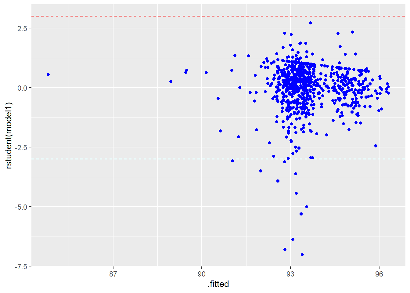
A residual plot is a graph used to detect violations of regression assumptions such as linearity, normality, and equal variances (homoscedasticity). It is typically formed by either graphing the predicted values \(\hat{y_i}\) (i.e. the fitted values) on the \(x\)-axis and the residuals \(e_i\) on the \(y-axis\).
An improved version of this is to use the studentized residuals \(r_{(-i)}\) (also known as jackknife residuals or rstudent residuals), which have been adjusted to have an approximate \(t\)-distribution with \(n-k-2\) df. These are the residuals that would be by leaving each observation out (this is the “jackknife” principle) and refitting the model, then finding and standardizing the residual from predicting the removed data value. This helps “unmask” outliers. You can get these in base R with the rstudent command.
A “rule of thumb” is to “flag” points for further scrutiny when the absolute value of the standardized residual exceeds 3, i.e. \[|r_{(-i)}| > 3\] There are also elaborate tables available with more exact critical values based on Bonferonni-corrected \(p\)-values of the \(t(n-k-2)\) distribution.
Heteroscedasticity (i.e. violation of equal variances): Checked with the Breusch-Pagan test or Levene’s test. A small \(p\)-value indicates a violation, similar to a funnel or horn-shaped pattern in a residual plot. Deleting outliers (if justifiable) or a transformation can help.
Non-normal residuals: Checked with the Shapiro-Wilk test. A small \(p\)-value indicates a violation, similar to a non-linear pattern in the normal probability plot (i.e. qq-plot). Deleting outliers (if justifiable) or a transformation can help.
Autocorrelated residuals. Checked with the Durbin-Watson test. A small \(p\)-value indicates a violation. This often happens when the predictor variable is time, and methods studied in time series analysis can help.
Multicollinearity. Checked with the largest VIF (variance inflation factor). \[VIF=\frac{1}{1-R_j^2}\] where \(R_J^2\) is the r-squared value that would be obtained with a regression of variable \(X_j\) as the response variable and all other \(X_i\)’s as the predictors. A \(VIF>10\) indicates multicollinearity (i.e. predictors that are highly correlated with each other). This can result in inflated standard errors (which will distort hypothesis tests, \(p\)-values, and confidence intervals) and inaccurate parameter estimates, including the “wrong signs” problem.
Outliers. Checked with Cook’s Distance (a measure of the influence of a point, briefly mentioned on page 173 of the text). We’ll use the “rule of thumb” where Cook’s \(D>0.5\) indicates an outlier.
3.6 Standardized Beta Coefficients
Some disciplines (particularly in the social sciences) want to standardize the regression coefficients (i.e. the betas). This is done especially when the various \(X\) variables are measured on very different scales, making it difficult to judge the various slopes solely on their magnitude.
The idea is that a one standard deviation increase in an \(X\) variable will have an impact of a certain number of standard deviations on the \(Y\) variable, given by the standardized beta coefficient, which I will call \(\hat{\beta_j}^*\).
It can be computed: \[\hat{\beta_j}^*=\hat{\beta_j} \frac{s_x}{s_y}\]
Note that this will NOT impact the test statistics or \(p\)-values that you would get from either Type I (sequential) tests that you get from the anova command or the Type II (unique) tests that you get from summary or Anova.
Many people think standardized betas are a bit silly and not worth the trouble, while others think they are absolutely necessary in any multiple regression analysis.
I demonstrated getting the standardized betas in two different ways:
standardizing all of the variables (i.e. centering by subtracting the mean and then dividing by the standard deviation) manually, except for categorical predictors
using a function
lm.betafrom thelm.betapackage to do this for you
The noted statistician Andrew Gelman believes that one should divide by 2 standard deviations, rather than 1, when standardizing for this reason, in order to make the standardized beta coefficients of the continuous predictors comparable with the beta coefficients for categorical predictors.
Read more about that here: stat.columbia.edu/~gelman/research/published/standardizing7.pdf
3.7 Effect Sizes
Hypothesis testing has been controversial for decades. Back when I was in graduate school, a book called “What If There Were No Signficiance Tests” was published, and similar papers were written before I was born. Recently, a journal in social psychology banned \(p\)-values from manuscripts submitted for publication there, and the American Statistical Association released a statements urging us to move beyond just looking at whether \(p < 0.05\).
https://amstat.tandfonline.com/doi/full/10.1080/00031305.2016.1154108
https://www.tandfonline.com/doi/full/10.1080/00031305.2019.1583913
In the social sciences, effect sizes have been popular for years as a measure of the size of an effect (the strength of a relatiohship), to either accompany or replace a probabilistic measure such as a \(p\)-value.
I’ll first demonstrate the idea of the effect size using a \(t\)-test, where the most common effect size measure is Cohen’s \(d\) (Jacob Cohen was a well-known quantitative psychologist).
\[d=\frac{\bar{x_1}-\bar{x_2}}{s_{pooled}}\]
This is just the standardized difference between the means. A rule of thumb is to classify this as a “small effect” at \(d=0.2\), “medium effect” at \(d=0.5\) and “large effect” when \(d=0.8\). Similar measures such as Glass’s \(\Delta\) and Hedges’s \(g\) exist.
In multiple regression and ANOVA models, there are several choices. We could just use the \(R^2\) or adjusted \(R^2\), or other variations including Cohen’s \(f^2\), \(\eta^2\), or \(\omega^2\). For \(R^2\) we are getting a measure for the entire model, while for the other statistics it is for a particular predictor variable \(X\). \(f^2\) is using the partial correlation between \(X\) and \(Y\) controlling for the other \(X\) variables.
\[f^2=\frac{r^2}{1-r^2}\]
\[R^2=\frac{SSModel}{SSTotal}\]
\[\eta^2=\frac{SSX}{SSTotal}\]
For convenience, here are all conventional effect sizes for all tests in the pwr package:
| Test | small |
medium |
large |
|---|---|---|---|
tests for proportions (p) |
0.2 | 0.5 | 0.8 |
tests for means (t) |
0.2 | 0.5 | 0.8 |
chi-square tests (chisq) |
0.1 | 0.3 | 0.5 |
correlation test (r) |
0.1 | 0.3 | 0.5 |
anova (anov) |
0.1 | 0.25 | 0.4 |
general linear model (f2) |
0.02 | 0.15 | 0.35 |
http://psychology.okstate.edu/faculty/jgrice/psyc3214/Ferguson_EffectSizes_2009.pdf (Christopher J. Ferguson’s article on effect sizes)
3.8 Home Prices data
The main data set here is GrinnellHouses from the Stat2Data package. It has data on \(n=929\) homes and 15 variables.
The pertinent variables are:
SalePrice: Sale price of the house (dollars)
LotSize: Lot size (in acres)
SquareFeet: The square footage of the home’s living space.
Bedrooms Number of bedrroms
Baths: Number of bathrooms
I created a binary version of YearBuilt called Old, based on being built before 1970.
data(GrinnellHouses)

Houses <- GrinnellHouses %>%
  dplyr::select(SalePrice,ListPrice,SPLPPct,SquareFeet,LotSize,Bedrooms,Baths,YearBuilt) %>%
  mutate(Old=(YearBuilt<1970)) %>%
  na.omit() %>%
  as_tibble()

print(Houses,width=Inf)
## # A tibble: 732 × 9
## SalePrice ListPrice SPLPPct SquareFeet LotSize Bedrooms Baths YearBuilt Old
## <int> <int> <dbl> <int> <dbl> <int> <dbl> <int> <lgl>
## 1 27000 35000 77.1 1224 0.172 3 1 1900 TRUE
## 2 30750 35000 87.9 1277 0.207 3 1 1900 TRUE
## 3 42000 45900 91.5 1079 0.199 3 1 1900 TRUE
## 4 50000 52500 95.2 912 0.218 3 2 1900 TRUE
## 5 50000 50000 100 1488 0.17 3 2 1900 TRUE
## 6 54000 71500 75.5 2160 0.313 4 1.75 1880 TRUE
## 7 54000 58900 91.7 1034 0.284 3 1.5 1900 TRUE
## 8 59000 62500 94.4 1008 0.284 2 1 1900 TRUE
## 9 60000 63000 95.2 1440 0.258 4 0.75 1954 TRUE
## 10 60500 69000 87.7 2105 0.230 4 2.75 1900 TRUE
## # ℹ 722 more rows## SalePrice ListPrice SPLPPct SquareFeet LotSize
## SalePrice 1.0000000 0.9946302 0.20507667 0.65240470 0.31779326
## ListPrice 0.9946302 1.0000000 0.12653092 0.67015911 0.34455439
## SPLPPct 0.2050767 0.1265309 1.00000000 -0.03760488 -0.06842539
## SquareFeet 0.6524047 0.6701591 -0.03760488 1.00000000 0.17911246
## LotSize 0.3177933 0.3445544 -0.06842539 0.17911246 1.00000000
## Bedrooms 0.4197103 0.4226686 0.04399417 0.53986039 0.08544781
## Baths 0.7030635 0.7135537 0.03446345 0.64260447 0.22365336
## YearBuilt 0.5010841 0.4925000 0.15088770 0.02393692 0.08690342
## Old -0.4616856 -0.4549292 -0.11609707 -0.14147749 -0.11865833
## Bedrooms Baths YearBuilt Old
## SalePrice 0.41971034 0.70306353 0.50108412 -0.4616856
## ListPrice 0.42266861 0.71355374 0.49250000 -0.4549292
## SPLPPct 0.04399417 0.03446345 0.15088770 -0.1160971
## SquareFeet 0.53986039 0.64260447 0.02393692 -0.1414775
## LotSize 0.08544781 0.22365336 0.08690342 -0.1186583
## Bedrooms 1.00000000 0.50794001 0.03367967 -0.1243224
## Baths 0.50794001 1.00000000 0.37305341 -0.4151798
## YearBuilt 0.03367967 0.37305341 1.00000000 -0.7259687
## Old -0.12432241 -0.41517976 -0.72596869 1.0000000## Old min Q1 median Q3 max mean sd n missing
## 1 FALSE 27100 125000 170000 245000 606000 193827.1 96712.80 205 0
## 2 TRUE 10900 75700 108000 137950 452000 112355.5 56987.11 527 0##
## Two Sample t-test
##
## data: SalePrice by Old
## t = 14.063, df = 730, p-value < 2.2e-16
## alternative hypothesis: true difference in means between group FALSE and group TRUE is not equal to 0
## 95 percent confidence interval:
## 70097.60 92845.55
## sample estimates:
## mean in group FALSE mean in group TRUE
## 193827.1 112355.5##
## Call:
## lm(formula = SalePrice ~ Old, data = Houses)
##
## Residuals:
## Min 1Q Median 3Q Max
## -166727 -43980 -10591 29770 412173
##
## Coefficients:
## Estimate Std. Error t value Pr(>|t|)
## (Intercept) 193827 4916 39.43 <2e-16 ***
## OldTRUE -81472 5794 -14.06 <2e-16 ***
## ---
## Signif. codes: 0 '***' 0.001 '**' 0.01 '*' 0.05 '.' 0.1 ' ' 1
##
## Residual standard error: 70380 on 730 degrees of freedom
## Multiple R-squared: 0.2132, Adjusted R-squared: 0.2121
## F-statistic: 197.8 on 1 and 730 DF, p-value: < 2.2e-16## Analysis of Variance Table
##
## Response: SalePrice
## Df Sum Sq Mean Sq F value Pr(>F)
## Old 1 9.7964e+11 9.7964e+11 197.75 < 2.2e-16 ***
## Residuals 730 3.6163e+12 4.9538e+09
## ---
## Signif. codes: 0 '***' 0.001 '**' 0.01 '*' 0.05 '.' 0.1 ' ' 1## [1] 0.2131536## # Effect Size for ANOVA
##
## Parameter | Cohen's f | 95% CI
## -----------------------------------
## Old | 0.52 | [0.46, Inf]
##
## - One-sided CIs: upper bound fixed at [Inf].## [1] 0.270896## # Effect Size for ANOVA
##
## Parameter | Eta2 | 95% CI
## -------------------------------
## Old | 0.21 | [0.17, 1.00]
##
## - One-sided CIs: upper bound fixed at [1.00].# try with different variable besides SalePrice
model1 <- lm(SPLPPct ~ SquareFeet + LotSize + Bedrooms + Baths + factor(Old) ,
data=Houses)
summary(model1)##
## Call:
## lm(formula = SPLPPct ~ SquareFeet + LotSize + Bedrooms + Baths +
## factor(Old), data = Houses)
##
## Residuals:
## Min 1Q Median 3Q Max
## -43.404 -2.388 1.034 3.855 17.341
##
## Coefficients:
## Estimate Std. Error t value Pr(>|t|)
## (Intercept) 94.3463877 1.0863257 86.849 < 2e-16 ***
## SquareFeet -0.0009551 0.0004932 -1.937 0.05318 .
## LotSize -0.1826619 0.0888763 -2.055 0.04021 *
## Bedrooms 0.5320880 0.3191707 1.667 0.09593 .
## Baths 0.2446987 0.4758423 0.514 0.60724
## factor(Old)TRUE -1.7019116 0.5901119 -2.884 0.00404 **
## ---
## Signif. codes: 0 '***' 0.001 '**' 0.01 '*' 0.05 '.' 0.1 ' ' 1
##
## Residual standard error: 6.402 on 726 degrees of freedom
## Multiple R-squared: 0.02703, Adjusted R-squared: 0.02033
## F-statistic: 4.034 on 5 and 726 DF, p-value: 0.001284## SquareFeet LotSize Bedrooms Baths factor(Old)
## 1.956708 1.059185 1.513656 2.256853 1.254172##
## Call:
## lm(formula = SPLPPct ~ SquareFeet + LotSize + Bedrooms + Baths +
## factor(Old), data = Houses)
##
## Residuals:
## Min 1Q Median 3Q Max
## -43.404 -2.388 1.034 3.855 17.341
##
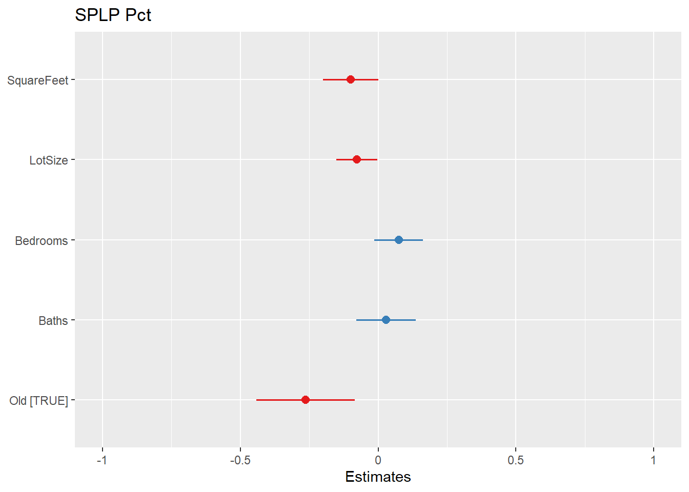
## Coefficients:
## Estimate Standardized Std. Error t value Pr(>|t|)
## (Intercept) 94.3463877 NA 1.0863257 86.849 < 2e-16 ***
## SquareFeet -0.0009551 -0.0991731 0.0004932 -1.937 0.05318 .
## LotSize -0.1826619 -0.0774334 0.0888763 -2.055 0.04021 *
## Bedrooms 0.5320880 0.0750853 0.3191707 1.667 0.09593 .
## Baths 0.2446987 0.0282814 0.4758423 0.514 0.60724
## factor(Old)TRUE -1.7019116 -0.1182393 0.5901119 -2.884 0.00404 **
## ---
## Signif. codes: 0 '***' 0.001 '**' 0.01 '*' 0.05 '.' 0.1 ' ' 1
##
## Residual standard error: 6.402 on 726 degrees of freedom
## Multiple R-squared: 0.02703, Adjusted R-squared: 0.02033
## F-statistic: 4.034 on 5 and 726 DF, p-value: 0.001284#look at x=age, y=aj
#unstandarized beta coefficient for age is beta.hat1 = -0.007775
#s_x = sd(Data$age) = 18.46676
#s_y = sd(Data$aj) = 2.766055
#beta.star1 = beta.hat1 * s_x/s_y = -0.0519
# effect sizes
rsquared(model1) ## [1] 0.02703303## Analysis of Variance Table
##
## Response: SPLPPct
## Df Sum Sq Mean Sq F value Pr(>F)
## SquareFeet 1 43.2 43.24 1.0552 0.304659
## LotSize 1 120.2 120.22 2.9338 0.087171 .
## Bedrooms 1 174.5 174.48 4.2577 0.039429 *
## Baths 1 147.8 147.81 3.6069 0.057936 .
## factor(Old) 1 340.9 340.86 8.3177 0.004042 **
## Residuals 726 29751.0 40.98
## ---
## Signif. codes: 0 '***' 0.001 '**' 0.01 '*' 0.05 '.' 0.1 ' ' 1## # Effect Size for ANOVA (Type I)
##
## Parameter | Cohen's f (partial) | 95% CI
## -----------------------------------------------
## SquareFeet | 0.04 | [0.00, Inf]
## LotSize | 0.06 | [0.00, Inf]
## Bedrooms | 0.08 | [0.01, Inf]
## Baths | 0.07 | [0.00, Inf]
## factor(Old) | 0.11 | [0.05, Inf]
##
## - One-sided CIs: upper bound fixed at [Inf].## # Effect Size for ANOVA (Type I)
##
## Parameter | Eta2 (partial) | 95% CI
## -------------------------------------------
## SquareFeet | 1.45e-03 | [0.00, 1.00]
## LotSize | 4.02e-03 | [0.00, 1.00]
## Bedrooms | 5.83e-03 | [0.00, 1.00]
## Baths | 4.94e-03 | [0.00, 1.00]
## factor(Old) | 0.01 | [0.00, 1.00]
##
## - One-sided CIs: upper bound fixed at [1.00].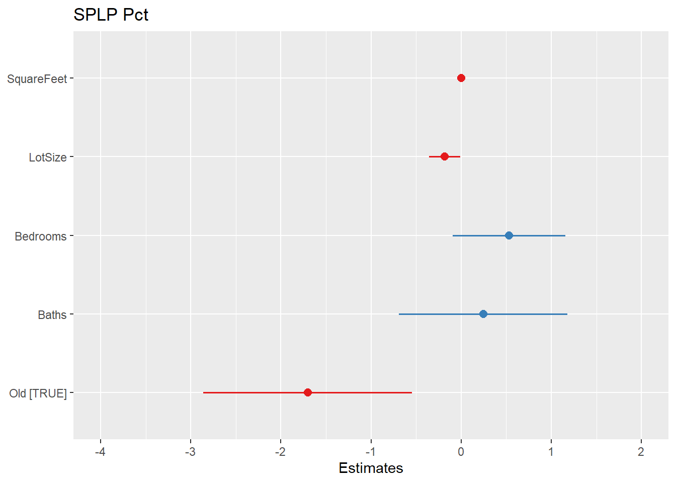

# residual plot of fitted vs studentized residuals
require(broom)
augment(model1) %>%
  ggplot(aes(x=.fitted,y=rstudent(model1))) + geom_point(col="blue") +
  geom_hline(yintercept=c(-3,3),color="red",linetype="dashed")